McGill MATH 264 tutoring

Point the right thumb upward. The curled fingers give the positive boundary direction, counterclockwise as viewed from positive $z$. Stokes requires an oriented smooth or piecewise-smooth surface, its compatible boundary direction and a continuously differentiable field on an open neighbourhood of the surface.

The disk is smooth with a smooth circular boundary; the polynomial field is continuously differentiable everywhere. Its curl is $\nabla\times\mathbf F=(0,0,2)$. Therefore

A direct boundary check uses $\mathbf r(t)=(2\cos t,2\sin t,1)$, $0\le t\le2\pi$. Then $\mathbf r'=(-2\sin t,2\cos t,0)$ and $\mathbf F(\mathbf r(t))\cdot\mathbf r'(t)=4$, again giving $8\pi$.

The disk is not a closed surface, so applying the divergence theorem to it would not calculate this circulation. Stokes relates circulation to curl flux, not to flux of $\mathbf F$ itself.

The compatible normal is now $(0,0,-1)$, and the circulation is $-8\pi$. A direct check with $\mathbf r_{\rm rev}(t)=(2\cos t,-2\sin t,1)$ gives dot product $-4$. Reversing only the boundary while retaining the upward normal would pair incompatible orientations.

When differentiating in $t$, treat $\sin x$ as constant. For $u_{xx}$, differentiate twice in $x$. Then substitute the boundary positions and the initial time independently.

The derivatives are

Thus $u_t=u_{xx}$ at every interior point. Since $\sin0=\sin\pi=0$, both boundary values are zero for all $t\ge0$. Finally, $e^0=1$, so $u(x,0)=\sin x$ across the whole interval. The initial profile also agrees with the zero endpoint data at $x=0,\pi$.

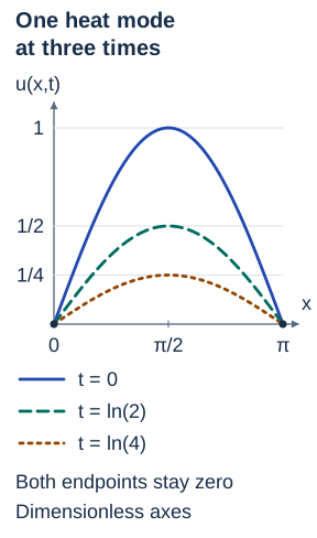
Now test $v(x,t)=2e^{-t}\sin x$. It satisfies the same PDE and both boundary conditions, but $v(x,0)=2\sin x$ fails the specified initial profile; for example, it gives $2$ rather than $1$ at $x=\pi/2$. A solution of the differential equation alone is not necessarily a solution of the full initial-boundary-value problem.

The sine profile keeps its zeros and its shape while its amplitude decays. This is a verification of a proposed solution, not yet a derivation of how to find it.

Each differentiation of the sine or cosine in $x$ contributes a chain-rule factor of $2$.

For $u=e^{-4t}\sin(2x)$, both $u_t$ and $u_{xx}$ equal $-4e^{-4t}\sin(2x)$. The endpoint sines vanish, and the time factor is $1$ at $t=0$. The first candidate matches the boundaries and initial data, but its PDE residual is $u_t-u_{xx}=3e^{-t}\sin(2x)$, which is not identically zero. It does not pass merely because that residual vanishes at some positions.

The boundary at the right end moved. Check it with the new sine, then compare the two derivatives.

Two spatial derivatives give $u_{xx}=-\tfrac14e^{-\lambda t}\sin(x/2)$; the time derivative gives $u_t=-\lambda e^{-\lambda t}\sin(x/2)$. Their equality requires $\lambda=1/4$. The endpoint values are zero because $\sin0=\sin\pi=0$, and at $t=0$ the required profile remains. Changing the interval can change the admissible spatial frequency and decay rate. Reusing $e^{-t}$ automatically would fail the PDE.

The PDE and zero boundary conditions are linear. Check each sine mode with its own time factor, then add the results. Linearity does not make their decay rates equal.

Both $u_t$ and $u_{xx}$ equal $$\begin{aligned}&-e^{-t}\sin x\\&\quad+18e^{-9t}\sin(3x)\end{aligned}$$. Both sine terms vanish at $x=0,\pi$; setting $t=0$ gives the stated initial profile. The shared-factor candidate $$\begin{aligned}w&=e^{-t}[\sin x\\&\qquad-2\sin(3x)]\end{aligned}$$ has $$\begin{aligned}w_t-w_{xx}&=-16e^{-t}\sin(3x)\end{aligned}$$, so it fails the PDE.

Independent retry: for initial profile $3\sin(2x)+\sin(4x)$ on the same interval, write and check a two-mode solution before opening the next answer.

Use $$\begin{aligned}u&=3e^{-4t}\sin(2x)\\&\quad+e^{-16t}\sin(4x)\end{aligned}$$. Both derivatives equal $$\begin{aligned}&-12e^{-4t}\sin(2x)\\&\quad-16e^{-16t}\sin(4x)\end{aligned}$$. The endpoint values vanish and at $t=0$ the desired initial profile is recovered. These are finite sums of smooth functions, so no interchange of an infinite sum and a derivative is needed.