Constrained Optimization: Feasible Sets and Lagrange Multipliers

1. Write the allowed set before differentiating

For an objective $f(x,y)$, the feasible set $S$ contains exactly the points satisfying every constraint and domain condition. A global minimum at $p\in S$ means $f(p)\le f(q)$ for every $q\in S$. A local minimum only compares feasible points sufficiently near $p$. Reverse the inequality for a maximum. An extremum value and the point where it occurs are different parts of the answer.

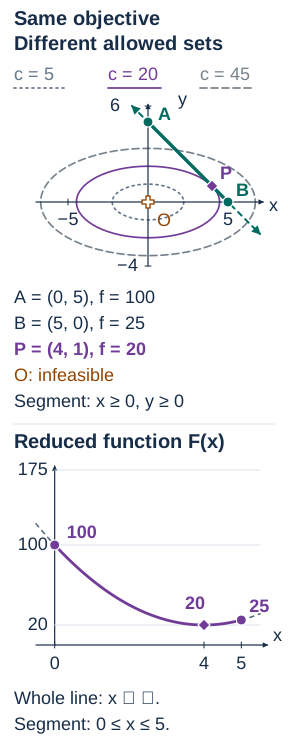
Compare three sets:

• $x+y=5$ is an entire line, with no nonnegativity restriction.
• $x+y=5,\ x\ge0,\ y\ge0$ is a closed segment, including two endpoints.
• $x^2+y^2\le4$ is a filled closed disk. The equation $x^2+y^2=4$ describes only its boundary circle.

A continuous function on a nonempty closed and bounded subset of $\mathbb R^2$ attains both a global minimum and a global maximum. This is a useful sufficient condition, not a requirement for every extremum. An unbounded set may still have a minimum; an open set may still contain one. If the theorem does not apply, examine the actual function and whether a proposed bound is attained.

In the procedure below, objectives are differentiable on a neighbourhood of the feasible set, except where a limitation is explicitly discussed. A more general problem also needs separate attention at points where the objective is undefined or not differentiable.

2. A line constraint: solve, then prove the global claim

Find the global extrema of

The unconstrained stationary point $(0,0)$ is not feasible. Do not use it as a constrained candidate.

Substitute $y=5-x$. Because the constraint is the entire line, $x$ ranges over all real numbers:

The square is nonnegative and equals zero only at $x=4$. Therefore the unique global minimum is $20$, attained at $(4,1)$. Also, $F(x)\to+\infty$ as $|x|\to\infty$, so there is no global maximum. The same identity proves both conclusions. Merely finding $F'(4)=0$ would not.

Change the allowed set

Add $x\ge0$ and $y\ge0$. Now $0\le x\le5$. The interior candidate still gives $20$; the endpoint values are

The global minimum remains $20$ at $(4,1)$, while the global maximum is now $100$ at $(0,5)$. Check completeness: the reduced derivative $F'(x)=10(x-4)$ vanishes only at $4$, and both endpoints have been included. Adding restrictions changed the maximum question.

3. What Lagrange multipliers actually establish

Suppose $f$ and $g$ are continuously differentiable near a feasible point $p$, and the equality constraint is $g(x,y)=c$. If $\nabla g(p)\ne\mathbf0$, every local extremum of $f$ along that regular constraint must satisfy

for some real number $\lambda$. These are necessary candidate equations. Solving them does not establish a minimum, maximum, existence or global conclusion by itself. A point with $\nabla f=\mathbf0$ is allowed: it can satisfy the equations with $\lambda=0$.

Why do parallel gradients appear? Along a differentiable feasible path $\mathbf r(t)$, the chain rule gives $\nabla g\cdot\mathbf r'(t)=0$. At a constrained local extremum, the derivative of $f(\mathbf r(t))$ is also zero. On a regular plane curve, both gradients are perpendicular to the tangent direction. Thus the objective cannot increase to first order along that tangent. Higher-order change may still matter.

For the previous line, use $g=x+y$, with $\nabla g=(1,1)\ne\mathbf0$. The equations are

Thus $x=4y$, giving $(4,1)$ and $\lambda=8$. This agrees with substitution. The completed square, rather than the multiplier value, proves the global minimum and absence of a maximum.

For the nonnegative segment, this regular-curve calculation supplies the interior candidate. The endpoints still need a separate check. They are endpoints of the feasible segment even though the supporting line is smooth.

4. A compact constraint can have several candidates

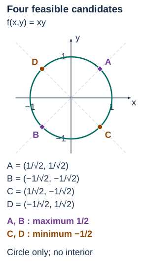
Find the extrema of $f(x,y)=xy$ on the unit circle $x^2+y^2=1$. The circle is nonempty, closed and bounded, and the polynomial objective is continuous, so both global extrema exist. Its constraint gradient $(2x,2y)$ never vanishes on the circle.

The candidate equations are

Avoid dividing by $x$ or $y$ before checking whether either can be zero. If $x=0$, the first equation gives $y=0$, contradicting the constraint. Likewise $y=0$ is impossible for a candidate. Multiply the first equation by $y$ and the second by $x$ to obtain $y^2=x^2$. The four candidates are

Same-sign coordinates give $f=1/2$; opposite signs give $f=-1/2$. Every global extremum must occur among these candidates because the circle has no endpoints or singular constraint points. Therefore the global maximum is $1/2$, attained at the two same-sign points, and the global minimum is $-1/2$, attained at the other two.

An independent check follows from $(x-y)^2\ge0$ and $(x+y)^2\ge0$: on the circle, $-1/2\le xy\le1/2$. Equality occurs at exactly the listed points. Finding a positive candidate alone would miss the minimum and the second maximum point.

5. A filled region needs interior and boundary checks

Find the extrema of

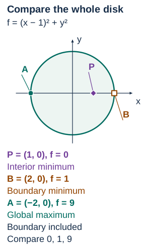
Continuity and compactness guarantee both global extrema. Partition the search into the interior of the disk and its boundary. Here “interior” means interior in the plane. A point on a constraint circle is not an interior point of a filled disk merely because it is not an endpoint of the circle.

Interior candidates

At a differentiable local extremum in the interior, $\nabla f=\mathbf0$. Thus

giving $(1,0)$. It lies strictly inside the disk and has value $0$.

Boundary candidates

On the circle $x^2+y^2=4$,

Since $-2\le x\le2$, the boundary minimum is $1$ at $(2,0)$, and its maximum is $9$ at $(-2,0)$.

The boundary multiplier equations give the same result:

If $y\ne0$, the second equation forces $\lambda=1$, and the first then says $-1=0$, impossible. Hence $y=0$, and the circle gives $x=\pm2$. This checks every case without silently dividing by a variable.

Compare the actual objective values

Compare $0$, $1$ and $9$. On the whole disk, the global minimum is $0$ at $(1,0)$, and the global maximum is $9$ at $(-2,0)$. The boundary minimum of $1$ is not the minimum on the filled disk. Restricting the problem to the circle would discard the true minimum.

For a region bounded by several smooth edges or arcs, inspect each boundary piece, its endpoints, corners and intersections. For example, a triangle requires its three edges and three vertices in addition to feasible interior stationary points. The circle calculation is not a complete recipe for every possible boundary. This lesson does not introduce general inequality-multiplier conditions.

6. A zero constraint gradient needs separate attention

The Lagrange conclusion above relies on $\nabla g\ne\mathbf0$. When this fails, do not conclude that no extremum exists.

Consider $f(x,y)=x$ with $g(x,y)=y^2-x^3=0$. The constraint implies $x\ge0$, and $(0,0)$ is feasible. Consequently the unique global minimum is $0$ at the origin. Yet

so no $\lambda$ satisfies $\nabla f=\lambda\nabla g$ there. A feasible parametrization $(x,y)=(t^2,t^3)$, $t\in\mathbb R$, gives $f=t^2$, confirming the minimum and showing that no global maximum exists. The zero constraint gradient marked a point that needed a direct check.

The chosen equation can also create a problem. Writing the line $x+y=5$ as $(x+y-5)^2=0$ leaves the feasible set unchanged, but the new constraint gradient vanishes everywhere on it. Return to the regular equation $x+y=5$ or substitute directly. A failed regularity hypothesis is not a verdict on the optimization problem.

7. A stationary candidate can still fail to be an extremum

On the regular constraint $y=0$, take $f(x,y)=x^3+y^2$. Lagrange gives $3x^2=0$, $2y=\lambda$, $y=0$, so $(0,0)$ is a candidate. Restricted to the line, however, $f(x,0)=x^3$. Arbitrarily near the origin there are positive and negative values. The candidate is neither a local minimum nor a local maximum along the line, and there is no global extremum on that line.

For comparison, $h(x,y)=x^4+y^2$ on the same line has $h(x,0)=x^4$, so the origin is its unique global minimum. Both reduced functions have second derivative zero at the origin. A zero second derivative is inconclusive; it does not mean “no extremum.” Use a sign comparison, a higher-order argument or another valid test.

Likewise, applying an unconstrained Hessian test without accounting for allowed directions does not classify a constrained problem. A constraint can remove directions used in an unconstrained comparison. For that distinct skill, use the existing unconstrained stationary-point practice and Hessian classification example, then return to the feasible set here. Those examples are on McGill course pages; they are supplementary topic links, not a claim of course equivalence.

8. Make the last line of the solution defensible

Before writing “minimum” or “maximum,” check:

1. Is the point feasible for every condition, including strict inequalities and the objective’s domain?
2. What guarantees existence, or what direct argument replaces that guarantee?
3. Have you included all relevant interior candidates, boundary pieces, endpoints, corners and points where a derivative or regularity condition fails?
4. Did your algebra keep all cases, including zero coordinates or zero multipliers?
5. Are you comparing values of the original objective, rather than multiplier values?
6. Does your argument establish a local result or a global one? If a bound is only approached, say it is not attained.

Try the guided practice, then return to MAST 218 tutoring. Bring the feasible-set sketch, your complete candidate list and the sentence that justifies your conclusion. A tutor can inspect those decisions before working through more algebra.

Course scope reference: Concordia’s current MAST 218 calendar description. The examples and teaching sequence above are original; the calendar is used only to establish topic scope.