McGill MATH 206 tutoring

The Hessian contains the second partial derivatives. A symmetric matrix $H$ is positive definite when $\mathbf d^{T}H\mathbf d>0$ for every nonzero displacement vector $\mathbf d$. Here $T$ denotes transpose.

The gradient equations are $4x+2y-6=0$ and $2x+4y=0$, giving $(x,y)=(2,-1)$ and $f=-6$. The symmetric Hessian is

Its eigenvalues are $6$ and $2$, both positive, so it is positive definite. Equivalently, for $\mathbf d=(u,v)^T$, $\mathbf d^TH\mathbf d=4u^2+4uv+4v^2=2(u+v)^2+2u^2+2v^2>0$ unless both components vanish. Positive curvature in every direction gives a strict local minimum.

For the global claim, write $u=x-2$, $v=y+1$. Direct expansion gives

This is positive for every nonzero displacement, so $-6$ is the unique global minimum value. A Hessian test at one point alone would not prove a global result for an arbitrary nonquadratic function.

The equations $4x+2y-6=0$, $2x-2y=0$ give $(1,1)$, with $g=-3$. Its Hessian is $\begin{pmatrix}4&2\\2&-2\end{pmatrix}$, whose determinant is $-12$, so it is indefinite and the point is a saddle. Directly, $g(1+t,1)=-3+2t^2$ while $g(1,1+t)=-3-t^2$. Arbitrarily near the stationary point there are both larger and smaller values.

For a candidate $c\mathbf a$, the residual is $\mathbf b-c\mathbf a$. Try making it orthogonal to $\mathbf a$. Remember that $\mathbf a\cdot\mathbf a=\lVert\mathbf a\rVert^2$, not $\lVert\mathbf a\rVert$. The denominator is positive because $\mathbf a\ne\mathbf0$.

The orthogonality equation is $\mathbf a\cdot(\mathbf b-c\mathbf a)=0$. Since $\mathbf a\cdot\mathbf b=6$ and $\mathbf a\cdot\mathbf a=5$, it gives $c_*=6/5$. Thus

Check the result: $\mathbf p\in L$ and $\mathbf a\cdot\mathbf r=14/5-14/5=0$. The scalar $c_*$, the projection vector $\mathbf p$, and the residual vector $\mathbf r$ are different objects.

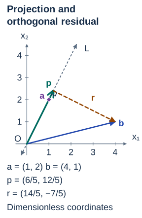
Orthogonality also proves optimality. For any real number $c$,

The cross term vanishes because $\mathbf r\cdot\mathbf a=0$. The added square is nonnegative and is zero only for $c=6/5$. Hence $\mathbf p$ is the unique closest vector, and the minimum distance is $\lVert\mathbf r\rVert=7/\sqrt5$. We minimized squared distance; it has the same minimizer as distance because square root is increasing on nonnegative numbers. A nonzero residual means $\mathbf b$ is not on the line, not that the projection failed.

Compute the dot product first. Zero projection does not require the input vector to be zero.

Now $\mathbf a\cdot\mathbf b=2-2=0$, so $c_*=0$, $\mathbf p=\mathbf0$, and $\mathbf r=(2,-1)^T$. The minimum distance is $\sqrt5$. Every nonzero move along $L$ adds a positive squared-distance term.

Both numerator and denominator change. Compare the product of coefficient and generator, not the coefficient alone.

The new coefficient is $(-12)/20=-3/5$. Multiplying gives $$\begin{aligned}&(-3/5)(-2,-4)^T\\&\quad=(6/5,12/5)^T\end{aligned}$$, the same projection. The residual and minimum distance are unchanged because the set of candidate vectors is unchanged. The coefficient depends on the chosen generator; the closest vector does not.

This is the same line-projection problem in $\mathbb R^3$. A zero residual would require all three target values to be the same.

The coefficient is $c_*=9/3=3$, the fitted vector is $(3,3,3)^T$, and the residual is $(-2,-1,3)^T$. Its dot product with $(1,1,1)^T$ is zero. The squared error is $14$, and for any $c$ the objective equals $14+3(c-3)^2$. This proves the minimum rather than merely locating a stationary point.

Independent retry: replace the targets by $(2,2,5)^T$. Find the fit and squared error before opening the next answer.

The minimizing constant is still $3$, but the residual is now $(-1,-1,2)^T$ and its squared norm is $6$. The same fitted vector can accompany different errors. This calculation uses ordinary unweighted Euclidean least squares; no probabilistic model has been assumed.