Demand Elasticity and Revenue

1. Turn a slope into percentage sensitivity

The derivative $q^{\prime}(p)$ measures how weekly demand changes when unit price changes. Here $q^{\prime}(p)=-4$: a one-dollar increase in unit price reduces weekly demand by four units. This is an exact change in this linear model. A slope measures a change in units; elasticity compares relative changes and has no units.

For a small price change $\Delta p$, let $\Delta q=q(p+\Delta p)-q(p)$ be the resulting change in weekly demand. The local approximation $\Delta q\approx q^{\prime}(p)\Delta p$ gives the first formula below. Multiplying either relative change by 100 expresses it as a percentage.

Define demand elasticity $E(p)$ using the positive convention below. Because demand is decreasing, $q^{\prime}(p)<0$, so the minus sign makes $E(p)>0$. An elasticity of $0.5$ means that a small 1% price increase produces approximately a 0.5% demand decrease. Under this convention, $E$ is positive for decreasing demand; the factor $-E$ predicts the demand decrease.

2. Connect elasticity to revenue

Weekly revenue $R(p)$, in dollars per week, is price times quantity sold: $R(p)=p\,q(p)$. Raising the price adds revenue on each unit sold, while the fall in demand removes sales. The product rule accounts for both effects.

The prime in $R^{\prime}(p)$ means differentiation with respect to price. Its units are dollars of weekly revenue per dollar of unit-price change. Since $p\,q^{\prime}(p)=-E(p)q(p)$, factoring gives the identity below. Demand is positive on our interval, so the sign of $R^{\prime}(p)$ is the sign of $1-E(p)$.

3. Compare three prices on the same demand line

Substitute $q^{\prime}(p)=-4$ to get $E(p)=4p/(240-4p)$, then simplify as below. The slope stays at $-4$, but elasticity changes because the starting price and starting demand change.

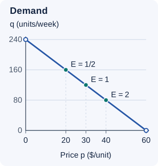
At $p=20$, demand is $160$ units per week and $E=1/2$. A small 1% price rise gives approximately a 0.5% demand fall. Revenue initially rises. At $p=40$, demand is only $80$ units and $E=2$: the same small 1% price rise gives approximately a 2% demand fall, so revenue initially falls.

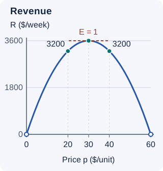
At $p=30$, demand is $120$ units and $E=1$. The revenue derivative is zero. In this model, $R^{\prime}(p)=240-8p$ is positive below 30 and negative above 30. Revenue therefore reaches its maximum at a price of 30 dollars per unit, with 120 units sold per week and weekly revenue of 3600 dollars.

One constant slope, three elasticity values

Revenue peaks where elasticity equals one in this model

4. Check the size of the price change

Unit elasticity at one price means zero instantaneous revenue change there. It does not mean that a finite price change leaves revenue unchanged. Let $h$ be a change in unit price from 30 dollars, with $-30<h<30$. Substitution gives the exact change below.

For example, raising the price from 30 to 31 dollars changes revenue from 3600 to 3596 dollars per week. The local estimate $R^{\prime}(30)\cdot1=0$ misses the four-dollar decrease. The horizontal tangent describes the first-order change at 30; the curved revenue graph still falls on either side.

An inelastic starting point also does not justify an arbitrarily large price rise. From $p=20$ to $p=50$, this model crosses the revenue maximum: revenue falls from 3200 to 2000 dollars per week. For a specified finite change, compare the two revenue values directly. Constant revenue on an entire interval requires $E(p)=1$ throughout that interval, not just at one price.