Improper Integrals: Define the Limit, Decide Convergence

1. What makes an integral improper?

The definite integral of a continuous function on a closed, bounded interval is ordinary, or proper. Two situations require a limiting definition here:

• An infinite bound: the interval continues without end.
• An unbounded integrand: near an endpoint or an interior point, the function being integrated can take values as large in absolute value as you like. Such a point is called a singularity here.

A missing value by itself does not force divergence. For example, a removable hole can be filled without changing an integral. A bounded jump can also be integrable in the ordinary sense. First inspect the domain and the behaviour near each excluded point.

For a right-infinite interval, assume that $f$ is continuous on every finite interval $[a,R]$. The definition is

$$\begin{aligned}&\int_a^\infty f(x)\,dx\\&\quad=\lim_{R\to\infty}\int_a^R f(x)\,dx.\end{aligned}$$

The symbol $\infty$ is not a number to substitute into an antiderivative. Evaluate the definite integral for finite $R$, then take a limit. For a left-infinite interval, use a separate finite lower bound:

$$\begin{aligned}&\int_{-\infty}^b f(x)\,dx\\&\quad=\lim_{L\to-\infty}\int_L^b f(x)\,dx.\end{aligned}$$

The improper integral converges if its defining limit is a finite real number. It diverges otherwise. A limit of $+\infty$ or $-\infty$ is divergence, and a limit that fails to exist because of oscillation is also divergence. For instance, the truncated integral $\int_0^R\cos x\,dx$ equals $\sin R$, which has no limit as $R\to\infty$.

2. An infinite interval, a finite limit

Worked example: how much area remains?

Determine whether $\int_1^\infty x^{-2}\,dx$ converges. For $R>1$, define the accumulated area $A(R)$:

$$\begin{aligned}A(R)&=\int_1^R x^{-2}\,dx\\&=\left[-\frac1x\right]_1^R\\&=1-\frac1R.\end{aligned}$$

Now take the limit:

$$\lim_{R\to\infty}A(R)=1.$$

Thus the improper integral converges to $1$. The curve stays positive forever, but the additional area becomes small enough for the total to approach a finite value.

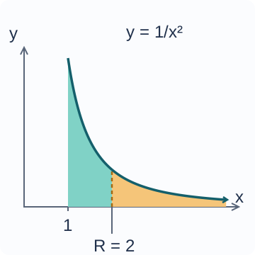
More generally, the tail after $R$ is

$$\int_R^\infty x^{-2}\,dx=\frac1R.$$

To make the omitted area at most $0.01$, choose $R\ge100$. This is an exact error bound for this particular example, not a general rule for all improper integrals.

Approaching zero is not enough

Compare with a slower-decaying function:

$$\int_1^R\frac{dx}{x}=\ln R.$$

Although $1/x\to0$, the accumulated area grows without bound. Therefore $\int_1^\infty dx/x$ diverges. A small function value far out on the axis does not by itself control the total area over an infinite interval.

3. An unbounded integrand near an endpoint

Suppose $f$ is continuous on $(a,b]$ and unbounded as $x\to a^+$. Approach the endpoint from inside the interval:

$$\begin{aligned}&\int_a^b f(x)\,dx\\&\quad=\lim_{t\to a^+}\int_t^b f(x)\,dx.\end{aligned}$$

For a singularity at the right endpoint instead, use

$$\begin{aligned}&\int_a^b f(x)\,dx\\&\quad=\lim_{t\to b^-}\int_a^t f(x)\,dx.\end{aligned}$$

These formulas apply to one problematic endpoint at a time. If both endpoints are problematic, split at an ordinary interior point and test the two pieces separately.

4. Split at every interior singularity

If $c$ lies inside $(a,b)$ and the function is unbounded near $c$, do not apply one antiderivative across the whole interval. Assuming no other improper points, define two separate quantities:

$$\begin{aligned}I_-&=\lim_{t\to c^-}\int_a^t f(x)\,dx,\\I_+&=\lim_{s\to c^+}\int_s^b f(x)\,dx.\end{aligned}$$

Only when both limits are finite does $\int_a^b f(x)\,dx=I_-+I_+$. If either piece diverges, the original improper integral diverges. The cutoffs $t$ and $s$ are independent.

An interior singularity can still be integrable

For a contrasting example, consider $\int_0^3|x-1|^{-1/2}\,dx$. Split at $1$. For $t<1$, the left truncated integral is

$$\begin{aligned}&\int_0^t\frac{dx}{\sqrt{1-x}}\\&\quad=2-2\sqrt{1-t}.\end{aligned}$$

It tends to $2$ as $t\to1^-$. For $s>1$, the right truncated integral is

$$\begin{aligned}&\int_s^3\frac{dx}{\sqrt{x-1}}\\&\quad=2\sqrt2-2\sqrt{s-1}.\end{aligned}$$

It tends to $2\sqrt2$ as $s\to1^+$. Both limits are finite, so the integral converges to $2+2\sqrt2$. The split is required even though the final answer is finite.

Two infinite bounds also need two checks

For $\int_{-\infty}^{\infty}f(x)\,dx$, choose a finite splitting point $c$ where the function is regular. If there are no finite singularities, test $\int_{-\infty}^c f(x)\,dx$ and $\int_c^\infty f(x)\,dx$ separately. Both must converge. A single symmetric limit from $-R$ to $R$ is not the defining test. Split at any finite singularities as well.

5. Why the two power tests differ

Power functions provide useful benchmarks. Let $p$ be real. For $p\ne1$,

$$\int_1^R x^{-p}\,dx=\frac{R^{1-p}-1}{1-p}.$$

As $R\to\infty$, the term $R^{1-p}$ tends to zero precisely when $p>1$. At $p=1$, the logarithm diverges. Hence

$$\begin{aligned}&\int_1^\infty\frac{dx}{x^p}<\infty\\&\quad\Longleftrightarrow p>1.\end{aligned}$$

In that convergent case, its value is $1/(p-1)$. Near zero, the same antiderivative gives a different limit:

$$\int_t^1 x^{-p}\,dx=\frac{1-t^{1-p}}{1-p}.$$

Now $t\to0^+$, so $t^{1-p}$ tends to zero when $p<1$. Thus

$$\begin{aligned}&\int_0^1\frac{dx}{x^p}<\infty\\&\quad\Longleftrightarrow p<1.\end{aligned}$$

Its value is then $1/(1-p)$. At $p=1$, this integral also diverges.

Keep the endpoint attached to the rule. At infinity, larger positive powers make the tail decay faster. Near zero, larger positive powers make the singularity stronger. Memorizing only “greater than one” loses the distinction.

In particular, $\int_0^\infty x^{-p}\,dx$ diverges for every real $p$: convergence would require both $p<1$ near zero and $p>1$ at infinity. A function with different behaviour at the two ends can still converge at both.

6. Compare when an antiderivative is unhelpful

For continuous nonnegative functions on a tail $[A,\infty)$, suppose $0\le f(x)\le g(x)$. Then:

• If $\int_A^\infty g(x)\,dx$ converges, the smaller integral of $f$ converges.
• If $\int_A^\infty f(x)\,dx$ diverges, the larger integral of $g$ diverges.

You can also compare the functions as you approach a finite singularity from one side, provided they are continuous on every closed interval on that side that stays away from the singularity. Closed, bounded intervals where the functions are continuous do not affect convergence. Use these comparisons only where both functions are nonnegative.

Choose the useful direction

To prove divergence of $\int_1^\infty dx/\sqrt{x^2+4}$, find a divergent lower bound. Since $x^2+4\le5x^2$ for $x\ge1$,

$$\frac1{\sqrt{x^2+4}}\ge\frac1{\sqrt5\,x}.$$

The lower-bound integral diverges like $\int_1^\infty dx/x$, so the original integral diverges. Merely bounding a function above by a divergent one would be inconclusive.

7. Four progressive questions

For each question, identify the improper point before calculating. State the limiting expression or comparison, then give a finite value when available or a clear convergence conclusion. Try the question before opening its hint or solution.

Logarithmic borderline cases: convergence and tail accuracy

A logarithm can change whether an infinite area converges, even when it changes the graph very slowly. This workshop goes beyond a yes/no answer: how far must a calculation extend before its omitted tail is small? These are original practice problems.

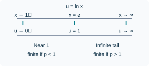
Turn the logarithm into the integration variable

For real $p$, consider $f_p(x)=1/[x(\ln x)^p]$ on $x>1$. Here $\ln x>0$, so every real power is defined and the integrand is positive. On finite bounds, the substitution $u=\ln x$, $du=dx/x$, gives

$$\int_e^B\frac{dx}{x(\ln x)^p}=\int_1^{\ln B}u^{-p}\,du,\qquad B>e.$$

Now take the limit. For $p\ne1$, the right side is $\big((\ln B)^{1-p}-1\big)/(1-p)$. For $p=1$, it is $\ln(\ln B)$. Therefore

$$\int_e^\infty\frac{dx}{x(\ln x)^p}\text{ converges exactly when }p>1.$$

When it converges, its value is $1/(p-1)$. At $p=1$ the growth is extremely slow but unbounded. A plot that appears to flatten is not a convergence proof.

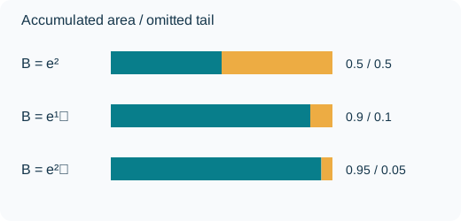
Worked example 1: a finite answer with a long tail

Approximate $I=\int_e^\infty dx/[x(\ln x)^2]$ by stopping at $B\ge e$. Find an exact error and a cutoff making that error at most $0.05$.

The substitution gives $I=\int_1^\infty u^{-2}\,du=1$. The truncated value and omitted tail are

$$I_B=1-\frac1{\ln B},\qquad R(B)=I-I_B=\frac1{\ln B}.$$

The integrand is positive, so $I_B$ is an underestimate and the absolute error is exactly $R(B)$. Solve $1/\ln B\le0.05$: since $\ln B>0$, this is $\ln B\ge20$, or $B\ge e^{20}\approx4.85\times10^8$. At $B=e^{10}$, the accumulated value is only $0.9$, with error $0.1$. Convergence alone does not tell you that a convenient finite cutoff is accurate.

Worked example 2: the same formula near a different endpoint

Determine when $J_p=\int_1^e dx/[x(\ln x)^p]$ is finite. The lower endpoint approaches 1 from the right. With $a>1$,

$$\int_a^e\frac{dx}{x(\ln x)^p}=\int_{\ln a}^1u^{-p}\,du.$$

As $a\to1^+$, the new lower bound tends to $0^+$, not infinity. The result is finite exactly when $p<1$, and then $J_p=1/(1-p)$. For $p=1$, $-\ln(\ln a)\to+\infty$; for $p>1$, the power expression also diverges to $+\infty$. For $p\le0$, the original function has a bounded continuous extension at 1, so this endpoint does not require a genuinely improper integral after extension; the same limiting result still holds.

For example, $p=1/2$ gives $J_{1/2}=2$, despite an unbounded integrand near 1. In contrast, the infinite-tail integral with $p=1/2$ diverges. Always identify which endpoint the substitution produces.

Four graduated questions

Check your reasoning: write finite bounds first, transform both bounds, and only then take the limit. If a comparison proves convergence, do not report an exact value unless you have separately calculated it.

Your next check

1. Mark every infinite bound and every point where the integrand becomes unbounded.
2. Split so that each piece has one improper end. Give each cutoff its own one-sided limit.
3. Evaluate the truncated integral, or justify a nonnegative comparison with the useful inequality direction.
4. Conclude convergence only when every piece has a finite limit. Add the values only then.

For a next step, compare this limiting-area reasoning with the series-convergence questions. A series sums discrete terms; an improper integral takes a limit of accumulated integrals. Their convergence tests are related, but a justification still needs the conditions of the test being used.

Official course context

Course description: current Concordia undergraduate calendar.