Integrating Factors for First-Order Linear ODEs

1. Recognize and normalize the equation

Let $x$ be the independent variable, $y=y(x)$ the unknown function, and $y^{\prime}=dy/dx$ its derivative. A first-order equation contains no derivatives higher than $y^{\prime}$. It is linear in $y$ if it can be written

$$a(x)y^{\prime}+b(x)y=c(x),$$

where $a$, $b$ and $c$ are known functions of $x$. The unknown function and its derivative appear only to the first power and are not multiplied together. For example, $y^{\prime}+xy=x^2$ is linear even though its coefficients depend on $x$; $y^{\prime}+y^2=x$ is nonlinear.

On an interval where $a(x)\ne0$, divide every term by $a(x)$:

$$\begin{gathered} y^{\prime}+p(x)y=q(x),\\ p=\frac{b}{a},\quad q=\frac{c}{a}. \end{gathered}$$

This is the standard form. Choose an open interval $I$ containing the initial input $x_0$ on which $p$ and $q$ are continuous. An initial condition $y(x_0)=y_0$ specifies the value the solution must have at that input. Under these conditions there is one solution for that initial value throughout $I$.

Quick normalization check. For $2y^{\prime}+4y=e^{-x}$, the coefficient needed by the integrating-factor formula is $p(x)=2$, and the right-hand side is $q(x)=e^{-x}/2$. Reading $p=4$ directly from the original equation skips the division.

2. Build the integrating factor from the product rule

We want a nonzero function $\mu(x)$, pronounced “mu”, such that multiplying the standard equation by $\mu$ gives a product derivative. Compare

$$\mu y^{\prime}+\mu p y=\mu q$$

with the product rule

$$(\mu y)^{\prime}=\mu y^{\prime}+\mu^{\prime}y.$$

The two left-hand sides match when $\mu^{\prime}=p\mu$. If $P(x)$ is any antiderivative of $p(x)$, then

$$\mu(x)=e^{P(x)}=e^{\int p(x)\,dx}$$

works: the chain rule gives $\mu^{\prime}=P^{\prime}e^P=p\mu$. Here $e$ is the base of the natural exponential. The exponential is positive, so dividing by $\mu$ later is allowed.

You may choose the simplest antiderivative $P$. Adding a constant to $P$ only multiplies $\mu$ by a nonzero constant, which does not change the resulting solution family. Any nonzero constant multiple of an integrating factor also works on the same interval.

Now integrate:

$$\begin{aligned}(\mu y)^{\prime}&=\mu q,\\ \mu y&=\int \mu(x)q(x)\,dx+C,\\ y&=\frac{\int \mu(x)q(x)\,dx+C}{\mu(x)}.\end{aligned}$$

The displayed integral stands for one antiderivative; $C$ is the arbitrary real integration constant. Keep that constant until the initial condition determines it. In particular, $\int p(x)y(x)\,dx$ is generally not $y(x)\int p(x)\,dx$: $y$ varies with $x$. The product rule is what makes the integration possible.

3. Solve a variable-coefficient initial-value problem

Find $y(x)$ for

$$\begin{gathered}xy^{\prime}+2y=x^2,\\ y(1)=1,\qquad x>0.\end{gathered}$$

Normalize and keep the interval

Divide by $x$, which is positive in this problem:

$$y^{\prime}+\frac{2}{x}y=x.$$

Thus $p(x)=2/x$, $q(x)=x$, and the interval is $(0,\infty)$. It contains the initial input $1$ and avoids division by zero.

Choose the factor and test the product

Since $x>0$, $\int 2/x\,dx=2\ln x$, where $\ln$ is the natural logarithm. Choose

$$\mu=e^{2\ln x}=x^2.$$

Multiplying the normalized equation by $x^2$ gives

$$x^2y^{\prime}+2xy=x^3.$$

The left side is $(x^2y)^{\prime}$, because the product rule gives $x^2y^{\prime}+2xy$. Writing out this one check prevents a sign or coefficient error from spreading.

Integrate, then apply the initial condition

$$\begin{aligned}x^2y&=\frac{x^4}{4}+C,\\ y&=\frac{x^2}{4}+\frac{C}{x^2}.\end{aligned}$$

At $x=1$, the condition is $1=1/4+C$, so $C=3/4$. The solution is

$$y(x)=\frac{x^2}{4}+\frac{3}{4x^2},\qquad x>0.$$

Check the equation and the condition separately

Differentiate: $y^{\prime}=x/2-3/(2x^3)$. Substitute into the original equation:

$$\begin{aligned}xy^{\prime}+2y&=\frac{x^2}{2}-\frac{3}{2x^2}\\ &\quad+\frac{x^2}{2}+\frac{3}{2x^2}\\ &=x^2.\end{aligned}$$

Also, $y(1)=1/4+3/4=1$. Both tests pass. A function can satisfy the differential equation but fail the initial condition; checking just one is not enough.

4. Read the family of solution curves

Before imposing $y(1)=1$, every function $y=x^2/4+C/x^2$ solves the equation on $x>0$. Changing $C$ changes the curve. At $x=1$, the family has value $1/4+C$, so exactly the member with $C=3/4$ passes through $(1,1)$.

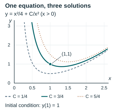
The equation itself gives the slope at the initial point: $y^{\prime}=x-2y/x=1-2=-1$. The selected curve therefore decreases just to the right of $x=1$, as the graph shows. A positive value of $y$ does not require a positive derivative.

The formula becomes unbounded as $x\to0^+$, because $3/(4x^2)\to+\infty$. This particular solution cannot extend continuously through zero. More generally, a zero of the original leading coefficient requires a fresh analysis; the normalized method alone does not decide whether a special solution can cross it.

5. Try three questions with explained answers

For each question, state the standard form and interval before integrating. Try the calculation before opening the answer.

6. Use the method on your next problem

1. Check linearity in the unknown function and its derivative.
2. Divide every term by the leading coefficient where it is nonzero. State an interval containing the initial input.
3. Read $p(x)$ from the normalized equation, choose $\mu=e^{\int p\,dx}$, and verify $\mu^{\prime}=p\mu$.
4. Rewrite the left side as $(\mu y)^{\prime}$, integrate, divide by $\mu$, and apply the initial condition.
5. Substitute into the original equation and check the initial value separately.

If the integration is the sticking point, revisit how to choose an integration method. For a shorter starting point, use the differential-equations solution check.

Working on a second-order equation with constant coefficients and a nonzero right-hand side? Continue with choosing a particular-solution trial. Check the equation type first; the first-order integrating-factor method above is a different procedure.

Course context and further reading

Concordia’s Fall 2026 ENGR 213 outline includes first-order linear equations and initial-value problems. McGill’s current MATH 263 description includes first-order ODEs. Use your current outline to choose the first-order equations and initial-value problems to practise. The questions here are original practice, not official assessment material.

• Concordia ENGR 213 Fall 2026 outline
• McGill Mathematics and Statistics course descriptions: MATH 263
• OpenStax Calculus Volume 2: First-Order Linear Equations