Line Integrals: Follow the Path and Its Direction

Nablio · 18 minPublished October 2, 2026

Stuck on a step? Text us Email us Request a lesson

For course topics and one-to-one help, see Concordia ENGR 233 tutoring.

How does a vector field contribute as you travel along a curve? A vector line integral adds the field’s signed contribution along each small displacement. We will build the calculation from a path, then test what changes when its parameter, direction or route changes.

Before starting, be comfortable differentiating coordinates, taking dot products and evaluating a definite integral. Review gradients and directional derivatives if those ideas are new. All coordinates, parameters and field components in this lesson are dimensionless real numbers; no force or physical unit is assumed.

1. Describe the path and its direction

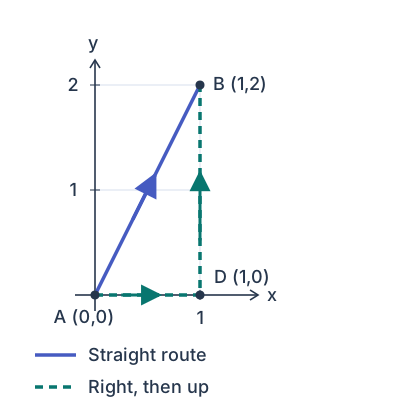
Start at $A=(0,0)$ and end at $B=(1,2)$ . The parameterization $\mathbf r(t)=(t,2t)$ , for $0\leq t\leq1$ , assigns a position to each value of $t$ . The parameter is a label that moves us along the route; it need not represent time.

Its two coordinates are $x(t)=t$ and $y(t)=2t$ . At $t=0$ we are at $A$ ; at $t=1/2$ , at $(1/2,1)$ ; and at $t=1$ , at $B$ . Increasing $t$ therefore traces the straight segment once from $A$ to $B$ . This choice of travel direction is the curve’s orientation.

A prime means differentiation with respect to the parameter. Differentiating both coordinates gives

$\mathbf r^{\prime}(t)=(1,2).$

This vector describes position change per unit change in $t$ . Over a small parameter increment $\Delta t$ , the displacement is approximately $\mathbf r^{\prime}(t)\Delta t$ ; here the approximation is exact because the path formula is linear. Its direction and magnitude will both matter.

Equal-scale coordinate axes show A at (0,0), B at (1,2), a straight path from A to B and a second path from A through D at (1,0) to B. Arrows mark both routes toward B. — The solid path follows $\mathbf r(t)$ . The dashed path first moves right to $D=(1,0)$ , then up to $B$ . The axes use the same scale. Shared endpoints alone do not guarantee equal line integrals.

2. Build the line integral

Consider the vector field $\mathbf F(x,y)=(2x,y)$ , defined on the whole plane $\mathbb R^2$ . A vector field assigns a vector to each point. First evaluate it at the points on the path:

$\mathbf F(\mathbf r(t))=(2t,2t).$

For a small displacement $\Delta\mathbf r$ , the dot product $\mathbf F\cdot\Delta\mathbf r$ measures the field’s contribution in the displacement direction. A component pointing along the displacement contributes positively, one pointing against it contributes negatively, and a perpendicular component contributes zero. Adding these local contributions and taking the limit gives the integral.

From vectors to an ordinary integral

Let $C$ denote the oriented segment from $A$ to $B$ . The notation $d\mathbf r$ represents an infinitesimal displacement along it. Substitution of $d\mathbf r=\mathbf r^{\prime}(t)\,dt$ gives

$\begin{aligned} &\int_C\mathbf F\cdot d\mathbf r\\ &=\int_0^1\mathbf F(\mathbf r(t))\cdot\mathbf r^{\prime}(t)\,dt\\ &=\int_0^1(2t,2t)\cdot(1,2)\,dt\\ &=\int_0^1 6t\,dt=3. \end{aligned}$

The dot product multiplies matching components and adds them: $(2t)(1)+(2t)(2)=6t$ . The definite integral then accumulates that contribution over the entire parameter interval. The result is a signed scalar, even though the field is vector-valued.

Keep the derivative’s magnitude. Replacing $\mathbf r^{\prime}(t)$ by a unit vector while keeping $dt$ would discard the displacement scale. If you choose to integrate with respect to arc length instead, the speed factor must appear in $ds=\lVert\mathbf r^{\prime}(t)\rVert\,dt$ .

These calculations assume a continuous field along a path that is smooth in pieces: a finite number of differentiable pieces with continuous derivatives. At a corner, calculate each piece separately and add the results. Our field is continuous everywhere, and both illustrated routes satisfy these conditions.

3. Check a potential before changing routes

A potential for $\mathbf F$ is a scalar function $\phi$ whose gradient equals the field. For this example, try $\phi(x,y)=x^2+y^2/2$ . Its partial derivatives are $\phi_x=2x$ and $\phi_y=y$ , so $\nabla\phi=(2x,y)=\mathbf F$ everywhere in the plane.

The chain rule explains why the endpoints now suffice:

$\frac{d}{dt}\phi(\mathbf r(t))=\nabla\phi(\mathbf r(t))\cdot\mathbf r^{\prime}(t).$

Integrating a derivative gives the change in its function. Since this potential is continuously differentiable on the whole plane, any piecewise-smooth route from $A$ to $B$ gives

$\begin{aligned}\int_C\mathbf F\cdot d\mathbf r &=\phi(B)-\phi(A)\\ &=\left(1^2+\frac{2^2}{2}\right)-0=3.\end{aligned}$

This field is conservative: the integral depends on the endpoints rather than the route between them. We established that property by verifying a potential, not by comparing just two paths.

Check the two-piece route directly

Use a new parameter $u$ on each piece, with $0\leq u\leq1$ . From $A$ to $D$ , take $\mathbf r_1(u)=(u,0)$ . Then $\mathbf F(\mathbf r_1(u))\cdot\mathbf r_1^{\prime}(u)=(2u,0)\cdot(1,0)=2u$ , so this piece contributes $1$ .

From $D$ to $B$ , take $\mathbf r_2(u)=(1,2u)$ . Now $\mathbf F(\mathbf r_2(u))\cdot\mathbf r_2^{\prime}(u)=(2,2u)\cdot(0,2)=4u$ , so this piece contributes $2$ . The total is $1+2=3$ , agreeing with the potential calculation.

Reversing direction changes the sign. Traveling from $B$ to $A$ gives $\phi(A)-\phi(B)=-3$ . Path independence keeps the ordered endpoints fixed. It does not remove orientation.

A domain check belongs in the method. For a planar field $(P,Q)$ with continuous first partial derivatives, the test $P_y=Q_x$ guarantees a potential on an open, simply connected domain, where every closed loop can be continuously shrunk to a point inside the domain. Equality alone is insufficient when these domain conditions are missing. Verifying an explicit potential on the whole domain used by the paths, as above, avoids that gap.

4. Try three variations

Attempt each question before opening its answer. Check the parameter interval and direction first, then choose the calculation.

Guided: same path, new parameter

Keep $\mathbf F(x,y)=(2x,y)$ , but describe the same segment by $\mathbf q(s)=(s/2,s)$ , for $0\leq s\leq2$ . Here $s$ is a parameter, not arc length. Verify the endpoints, find $\mathbf q^{\prime}(s)$ , and evaluate the vector line integral directly. Should it still equal $3$ ?

Show the answer and reasoning

Check the same oriented route
We have $\mathbf q(0)=A$ , $\mathbf q(2)=B$ and $y=2x$ , so the route and orientation agree with the original. The derivative is $\mathbf q^{\prime}(s)=(1/2,1)$ .
Keep the new derivative and bounds together
The field along the path is $\mathbf F(\mathbf q(s))=(s,s)$ . Therefore
$\begin{aligned} &\int_0^2(s,s)\cdot(1/2,1)\,ds\\ &=\int_0^2\frac{3s}{2}\,ds\\ &=3. \end{aligned}$
The smaller derivative is balanced by the longer parameter interval. A continuously differentiable, one-to-one, orientation-preserving change of parameter leaves the vector line integral unchanged.

Diagnose: reversing the route

A student travels from $B$ back to $A$ using $\mathbf p(t)=(1-t,2-2t)$ , for $0\leq t\leq1$ , and writes $\mathbf p^{\prime}(t)=(1,2)$ . Find the error and calculate the integral of $\mathbf F$ along this reversed path. Check it with the potential.

Show the answer and reasoning

Differentiate the actual path
Both coordinates decrease with $t$ , so $\mathbf p^{\prime}(t)=(-1,-2)$ . Reusing $(1,2)$ would keep the old direction. The field along this reversed route is $(2-2t,2-2t)$ .
Check the sign in two ways
$\begin{aligned} &\int_0^1\begin{pmatrix}2-2t\\2-2t\end{pmatrix}\cdot\begin{pmatrix}-1\\-2\end{pmatrix}\,dt\\ &=\int_0^1(-6+6t)\,dt\\ &=-3. \end{aligned}$
The potential gives $\phi(A)-\phi(B)=0-3=-3$ . The same geometric segment traversed in the opposite direction reverses the sign of this vector line integral.

Independent: do two routes always agree?

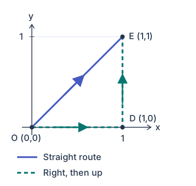
Change the field to $\mathbf G(x,y)=(-y,x)$ , defined on $\mathbb R^2$ , and use new endpoints $O=(0,0)$ and $E=(1,1)$ . Compare the straight route $\mathbf a(t)=(t,t)$ , $0\leq t\leq1$ , with the route that goes right to $D=(1,0)$ and then up to $E$ . Parameterize both pieces of the second route and compute both integrals. What do their values show?

Equal-scale axes show O at (0,0), E at (1,1), a straight route from O to E, and a two-piece route right through D at (1,0) then up to E. Arrows show the same start and end for both routes. — Use the same endpoints and orientation for a fair comparison. The field is now $\mathbf G=(-y,x)$ ; the potential found for $\mathbf F$ cannot be reused.

Show the answer and reasoning

Compute the straight route
Here $\mathbf a^{\prime}(t)=(1,1)$ and $\mathbf G(\mathbf a(t))=(-t,t)$ . Their dot product is $-t+t=0$ , so the straight route gives $0$ . The field is perpendicular to the displacement along this route.
Add the two other pieces
For each piece let $0\leq u\leq1$ . On $\mathbf b(u)=(u,0)$ , the dot product is $(0,u)\cdot(1,0)=0$ , giving $0$ . On $\mathbf c(u)=(1,u)$ , it is $(-u,1)\cdot(0,1)=1$ , giving $1$ . The two-piece total is $1$ .
State what the comparison proves
The same ordered endpoints give different values, $0$ and $1$ , so this field is path dependent. It cannot have a potential on the whole plane. The partial-derivative check agrees: for $P=-y$ and $Q=x$ , we have $P_y=-1\ne1=Q_x$ . One matching pair of routes would not establish path independence; one differing pair disproves it.

Use the method on your next problem

Mark the start and end, choose the parameter interval, and check the orientation.
Evaluate the field on the path and differentiate the path with respect to that same parameter.
Take the dot product before integrating. Split the path at corners.
If using a potential, verify its gradient and domain; subtract the starting value from the ending value.

For a refresher on gradients, return to the gradient and directional-derivative lesson. To place this topic in the wider course, use the Concordia ENGR 233 course guide.

Course context and further reading

This original Nablio lesson supports the line-integral part of ENGR 233. It does not cover surface integrals or the Green, Stokes and divergence theorems, reproduce an official exam, or predict assessed questions.

Useful for

Work on the step you’re missing.

Tell us the subject and your preferred time. Nablio confirms the details by text or email.

Request a lesson

Line Integrals: Follow the Path and Its Direction

1. Describe the path and its direction

2. Build the line integral

From vectors to an ordinary integral

3. Check a potential before changing routes

Check the two-piece route directly

4. Try three variations

Guided: same path, new parameter

Check the same oriented route

Keep the new derivative and bounds together

Diagnose: reversing the route

Differentiate the actual path

Check the sign in two ways

Independent: do two routes always agree?

Compute the straight route

Add the two other pieces

State what the comparison proves

Use the method on your next problem

Course context and further reading

Useful for

Work on the step you’re missing.