Marginal Cost: From an Estimate to an Exact Change

Worked example

Differentiate the model: $$\begin{gathered}C^\prime(q)=12+0.08q,\\C^\prime(50)=16.\end{gathered}$$ At 50 units, total cost is increasing at 16 CAD per unit. The fixed 500 CAD vanishes from the derivative because it does not vary with production.

For one extra unit, the derivative gives the estimate $16\times1=16$ CAD. Direct evaluation gives $$\begin{gathered}C(51)-C(50)\\=1216.04-1200\\=16.04.\end{gathered}$$ The exact cost of that extra unit is slightly larger because marginal cost increases between 50 and 51.

At 50 units, total cost is $1200$ CAD and average unit cost is $1200/50=24$ CAD per unit. Those are different quantities from the marginal rate of 16 CAD per unit.

Worked example

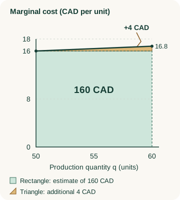
From 50 to 60 units, $h=10$. The local estimate is $$\begin{gathered}C^\prime(50)\times10\\=16\times10\\=160\text{ CAD}.\end{gathered}$$ The exact model gives $$\begin{gathered}C(60)-C(50)\\=1364-1200\\=164\text{ CAD}.\end{gathered}$$ The estimate is 4 CAD too low.

The graph below shows why. Across these ten units, marginal cost rises from $16$ to $16.8$ CAD per unit. The rectangle uses the starting rate; the thin triangle above it accounts for the missed increase.

Expanding the quadratic gives an exact check for any allowed increment: $$\begin{gathered}C(q+h)-C(q)\\=(12+0.08q)h+0.04h^2\\=C^\prime(q)h+0.04h^2.\end{gathered}$$ For this model, the amount missed by the linear estimate is $0.04h^2$ CAD. Increasing the batch from one unit to ten increases that error from 0.04 CAD to 4 CAD, a factor of 100. This error formula belongs to this quadratic; it is not a universal marginal-cost rule.

Worked example

For the same increase from 50 to 60 units, an antiderivative of $12+0.08q$ is $12q+0.04q^2$. Check it by differentiation, then evaluate upper minus lower: $$\begin{gathered}\int_{50}^{60}(12+0.08q)\,dq\\=[12q+0.04q^2]_{50}^{60}\\=864-700\\=164\text{ CAD}.\end{gathered}$$ This agrees with the direct cost difference and the graph’s full shaded area.

To find the total at 60 units, start at zero production and add the fixed cost: $$\begin{gathered}C(60)\\=C(0)+\int_0^{60}C^\prime(q)\,dq\\=500+864\\=1364\text{ CAD}.\end{gathered}$$ The integral from 50 to 60 alone gives 164 CAD, not 1364 CAD.

Units provide a check: CAD per unit multiplied by an increment in units gives CAD. A constant added to every total cost changes neither the derivative nor a cost difference. That is why marginal cost alone cannot determine the fixed cost.

Worked example

Worked example: compare totals and averages. At 50 units, $C(50)=1200$ CAD and $A(50)=1200/50=24$ CAD per unit. At 60 units, $C(60)=1364$ CAD and $$\begin{gathered}A(60)\\=1364/60\\=341/15\\\approx 22.73\end{gathered}$$ CAD per unit. Total cost rises by 164 CAD, while average unit cost falls by $19/15\approx1.27$ CAD per unit. Both production levels lie in the model’s domain.

Explain the change using the added batch. The ten extra units cost 164 CAD in total, or $164/10=16.40$ CAD per added unit. That is below the previous average of 24 CAD per unit. Combining the earlier 50 units and the new ten gives $$\begin{gathered}A(60)\\=\frac{50\times24+10\times16.40}{60}\\\approx22.73\end{gathered}$$ CAD per unit. The cheaper added batch pulls the overall average down. Its exact average cost is 16.40 CAD per unit; the starting marginal rate is $C^\prime(50)=16$ CAD per unit.

Now explain the local behaviour with a derivative. Dividing the model by q first gives $A(q)=500/q+12+0.04q$ for $0<q\le 200$. Differentiate: $A^\prime(q)=-500/q^2+0.04$. At $q=50$, $A^\prime(50)=-0.16$ CAD per unit squared. This measures the local change in average unit cost per additional unit of output. Meanwhile $C^\prime(50)=16$ CAD per unit is positive: the total is increasing locally while the average is decreasing locally.

A useful general check follows from the quotient rule: $$\begin{gathered}A^\prime(q)\\=\frac{qC^\prime(q)-C(q)}{q^2}\\=\frac{C^\prime(q)-A(q)}q\end{gathered}$$, wherever C is differentiable and $q>0$ is an interior point of the domain. Because q is positive, a marginal cost below average cost makes A′ negative; a marginal cost above average cost makes A′ positive. Equality gives a zero derivative. It does not by itself prove a minimum. These are local conclusions; for a specified finite batch, compare the actual averages or the exact batch cost.

Guided retry. Reuse $D(q)=300+8q+0.02q^2$ CAD, with q treated continuously on $0\le q\le 150$. Define $B(q)=D(q)/q$ for $0<q\le150$. At $q=40$, first write $B(40)=D(40)/40$ and D′(40). Then complete $$\begin{gathered}B^\prime(40)\\=[D^\prime(40)-B(40)]/40\end{gathered}$$. Before reading on, predict whether total cost and average unit cost rise or fall locally.

Guided check. $D(40)=652$ CAD, $B(40)=16.30$ CAD per unit and $D^\prime(40)=9.60$ CAD per unit. Thus $$\begin{gathered}B^\prime(40)\\=(9.60-16.30)/40\\=-0.1675\end{gathered}$$ CAD per unit squared. Total cost increases locally, while average unit cost decreases locally. A positive marginal cost tells you that the total is rising; comparing it with the average tells you the direction of the average’s local change.