Separable differential equations: keep the solutions you divide out

What to know first

You need basic derivatives and antiderivatives, the chain rule, exponentials and natural logarithms. A prime denotes differentiation with respect to the independent variable. The symbol $\ln$ means natural logarithm, and $C$ denotes an arbitrary real integration constant.

If integration is the obstacle, use choosing an integration method. That lesson already explains substitution and partial fractions. Here we use those tools to solve an equation for an unknown function.

1. Recognize a separable equation

An equation is separable when it can be written, on its stated domain, as

$$\frac{dy}{dx}=f(x)g(y).$$

The right side is a function of $x$ multiplied by a function of $y$. For example, $y'=2x(y-3)$ is separable. So is $y'=x^2$: take $g(y)=1$.

By contrast, the right side of $y'=x-y$ is a sum whose terms cannot be separated into one such product on an open region. Do not write $dy/y=(x-1)\,dx$: dividing $x-y$ by $y$ gives $x/y-1$. This equation has the linear form $y'+y=x$, so use the integrating-factor lesson.

The categories can overlap. The equation $y'=2y$ is both separable and linear. Choose a method because its steps are valid, rather than assuming every first-order equation has the same method.

2. Check constant solutions before dividing

For $y'=f(x)g(y)$, a value $a$ with $g(a)=0$ is a candidate constant solution $y(x)=a$. Substitute it into the original equation, and check that the equation is defined there. Such a constant solution is called an equilibrium solution.

For $y'=2x(y-3)$, the constant function $y=3$ works: its derivative and the right side are both zero for every $x$. Dividing by $y-3$ would exclude it from the following algebra, so record it first.

The factor $2x$ also vanishes at $x=0$. That says every solution has zero derivative at that particular input. It does not say every solution is constant on an interval.

Now work on an interval where $g(y(x))\ne0$. There,

$$\begin{gathered}\frac{y'}{g(y)}=f(x), \\ \int\frac{1}{g(y)}\,dy=\int f(x)\,dx.\end{gathered}$$

Why does the left integral use $dy$? If $H'(y)=1/g(y)$, the chain rule gives

$$\frac{d}{dx}H(y(x))=\frac{y'(x)}{g(y(x))}.$$

Separation is a convenient notation for this chain-rule calculation. Do not integrate $y$ as though it were a constant with respect to $x$.

Keep one integration constant after combining the constants from both sides. An implicit relation is acceptable when isolating $y$ is inconvenient, provided it defines the required differentiable branch and you check it in the original equation.

3. Work through an initial value

Solve

$$\begin{gathered}y'=2x(y-3), \\ y(0)=5.\end{gathered}$$

Keep the excluded case

The equilibrium $y=3$ solves the equation, but it does not satisfy $y(0)=5$. For the branch through the prescribed point, begin where $y-3\ne0$:

$$\frac{dy}{y-3}=2x\,dx.$$

Integrate with the correct logarithm

$$\ln|y-3|=x^2+C.$$

The absolute value allows either sign of $y-3$. Differentiating $\ln|y-3|$ along a nonzero branch gives $y'/(y-3)$.

Apply the initial condition

At $x=0$, $y=5$, so $C=\ln2$. On the branch through this point, $y-3$ is positive. Hence

$$\begin{gathered}y-3=2e^{x^2}, \\ y=3+2e^{x^2}.\end{gathered}$$

More generally, exponentiating the logarithmic relation gives $y=3+Ae^{x^2}$ with a nonzero signed constant $A$. The value $A=0$ is justified separately by the equilibrium check, not by claiming $e^C=0$. With it included, this family covers the equilibrium as well.

Verify the equation and the interval

$$\begin{gathered}y'=4xe^{x^2}, \\ 2x(y-3)=4xe^{x^2}, \\ y(0)=5.\end{gathered}$$

The solution is defined and differentiable for every real $x$, and $y-3=2e^{x^2}>0$. Its maximal interval is $\mathbb R$. There is no lost crossing through the divided-out value in this solution.

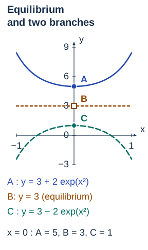
Try a changed initial value: what if $y(0)=1$? The answer is $y=3-2e^{x^2}$, still defined on $\mathbb R$. A negative value of $y-3$ is allowed. It is precisely why the absolute value and signed constant matter.

4. Interpret a growth model

In a simplified continuous model, a community has population $P(t)$, measured in people, at time $t$, measured in years. Suppose the growth rate is proportional to its current population:

$$\begin{gathered}P'=0.04P, \\ P(0)=1500.\end{gathered}$$

The coefficient has units $\mathrm{year}^{-1}$; therefore the right side has units people per year. It is a constant relative growth rate, not an addition of 0.04 people per year.

First, $P=0$ is an equilibrium. For the positive initial population, separation gives $dP/P=0.04\,dt$. A definite-integral form makes the initial value especially clear:

$$\int_{1500}^{P(t)}\frac{1}{u}\,du =\int_0^t0.04\,ds,$$

$$\begin{gathered}\ln\left(\frac{P(t)}{1500}\right)=0.04t, \\ P(t)=1500e^{0.04t}.\end{gathered}$$

The ratio inside the logarithm is dimensionless. Direct differentiation returns $0.04P(t)$, and substitution at zero returns 1500. The formula is mathematically defined for all real time; the stated forward model uses $t\ge0$.

The doubling time satisfies $e^{0.04t}=2$, so

$$t=\frac{\ln2}{0.04}\approx17.33\text{ years}.$$

After one year the multiplier is $e^{0.04}\approx1.04081$. A continuous relative rate of 0.04 per year therefore gives an effective one-year increase of about 4.081%, rather than exactly 4%.

The model predicts unbounded growth as $t\to\infty$. That is a property of the assumptions. It is not evidence that a real population can grow without limits.

5. Keep the interval containing the initial point

A formula may solve an equation on several disconnected intervals. An initial-value solution belongs on an interval containing its initial input; it cannot jump over a singularity.

Consider

$$\begin{gathered}y'=y^2, \\ y(0)=1.\end{gathered}$$

The equilibrium $y=0$ does not meet the initial value. For $y\ne0$, separation and integration give

$$\begin{gathered}\int y^{-2}\,dy=\int dt, \\ -\frac1y=t+C.\end{gathered}$$

The initial condition yields $C=-1$, so

$$y(t)=\frac1{1-t}.$$

Its derivative is $1/(1-t)^2=y^2$, but the formula is undefined at $t=1$. The maximal solution interval containing zero is $(-\infty,1)$. For forward time, it is $[0,1)$. The expression also satisfies the equation on $(1,\infty)$, but that separate branch is not a continuation through the infinite blow-up.

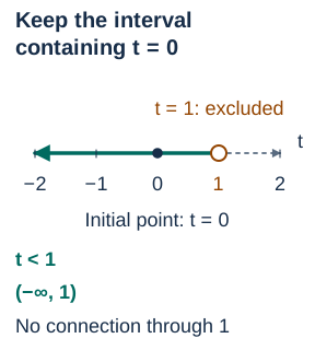
Check three things: restrictions already in the original equation, restrictions introduced while solving, and the selected solution’s own singularities. These may differ. For example, $y'=t/y$ excludes $y=0$ in the original equation; multiplying by $y$ does not make zero an admissible equilibrium.

6. Optional extension: growth with a limiting population

Use this section if logistic growth is in your assigned material or you want a further application. The official Dawson evidence establishes separation of variables, not logistic growth in every section.

Suppose a simplified population model uses

$$\begin{gathered}P'=0.3P\left(1-\frac{P}{600}\right), \\ P(0)=100.\end{gathered}$$

Time is measured in years, population in people, and 600 people is the model’s carrying capacity. The coefficient 0.3 has units $\mathrm{year}^{-1}$. The extra factor reduces the relative growth rate as the population approaches 600.

Find the equilibria and the sign

Both $P=0$ and $P=600$ are equilibrium solutions. For $0<P<600$, the right side is positive. For $P>600$, it is negative. These signs predict growth below capacity and decline above it. At either equilibrium, $P(1-P/600)=0$, so division by this product is invalid.

Separate on the branch between the equilibria

For $0<P<600$,

$$\frac{dP}{P(1-P/600)}=0.3\,dt,$$

$$\frac{1}{P(1-P/600)} =\frac1P+\frac1{600-P}.$$

Check the identity by combining the fractions. The second antiderivative has a minus sign because $d(600-P)/dP=-1$:

$$\ln\left(\frac{P}{600-P}\right)=0.3t+C.$$

Here the ratio is positive and dimensionless. The initial value gives $C=\ln(1/5)$. Thus

$$\begin{gathered}\frac{P}{600-P}=\frac15e^{0.3t}, \\ P(t)=\frac{600}{1+5e^{-0.3t}}.\end{gathered}$$

The denominator is positive for every real $t$, and the formula stays strictly between zero and 600. It therefore validates the branch used in separation. Its mathematical interval is $\mathbb R$; the forward population model uses $t\ge0$.

Check and interpret

Writing $D=1+5e^{-0.3t}$ temporarily,

$$P'=\frac{900e^{-0.3t}}{D^2},$$

$$\begin{aligned}&0.3P\left(1-\frac P{600}\right)\\&=0.3\frac{600}{D}\frac{5e^{-0.3t}}{D}\\&=\frac{900e^{-0.3t}}{D^2}.\end{aligned}$$

Also $P(0)=100$, and $P(t)\to600$ as $t\to\infty$. It approaches capacity without reaching it at any finite time. It reaches 300 people when $5e^{-0.3t}=1$, or $t=\ln5/0.3\approx5.365$ years. For comparison, the exponential model with the same initial value and coefficient would be $100e^{0.3t}$, with no capacity limit. Its coefficient is the same, but its initial absolute growth rate is 30 people per year; the logistic model starts at 25.

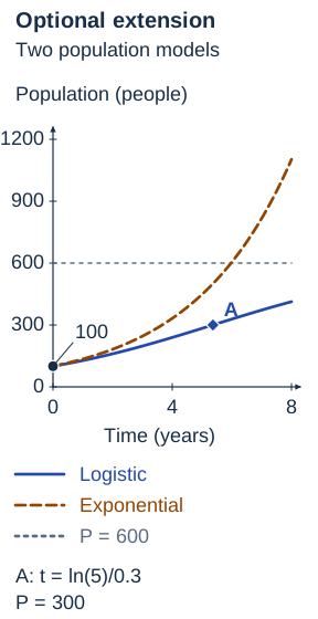
The explicit formula derived by dividing misses $P=0$. The family $600/(1+Ae^{-0.3t})$ recovers $P=600$ when $A=0$, but both equilibria must still be checked directly. For other initial values, inspect the denominator and interval again; do not carry this positive-denominator conclusion over automatically.

Optional application: a temperature approaches its surroundings

The official Dawson mathematics supplements include verifying solutions and separating variables under differential calculus (201-SN2-RE). This original application practises those methods; it is not evidence that Newton’s cooling model is required in every section. Use your current outline to choose the depth you need.

We approximate an object by a single uniform temperature $T(t)$, in degrees Celsius, at time $t$, in minutes. The surrounding temperature $A$ stays constant over the interval. Assume the temperature-change rate is proportional to the difference from the surroundings:

The constant $k$ has units $\mathrm{min}^{-1}$; the right side has units °C/min. This simplified model assumes internal temperature differences can be neglected and the effective heat-transfer conditions stay fixed. A real object with uneven temperatures, changing airflow or a phase change may not obey it. We do not predict such cases with this formula.

First check the equilibrium: $T=A$ gives zero on both sides. If $T(0)=T_0\ne A$, separation on the initial branch gives

The logarithm contains a dimensionless ratio, and $kt$ is dimensionless. The temperature excess $T-A$ keeps its initial sign, so

Directly, $T'=-k(T_0-A)e^{-kt}=-k(T-A)$, and $T(0)=T_0$. This formula also covers the separately checked equilibrium when $T_0=A$. Above the surroundings, the object cools; below them, it warms. At every finite forward time, a non-equilibrium solution stays strictly on its original side of $A$. It approaches $A$ as $t\to\infty$, rather than reaching or crossing it.

Worked examples: calibrate the model, then change the surroundings

1. Fit the excess, not the Celsius reading

An idealized object starts at $80\,^{\circ}\mathrm C$ in surroundings held at $20\,^{\circ}\mathrm C$. After 5 min it is at $50\,^{\circ}\mathrm C$. Treat these values as exact for this exercise. The initial excess is 60 °C and the later excess is 30 °C, so

Here 5 denotes the numerical time in minutes. The ratio $50/80$ would be wrong: the model makes the excess above 20 decay exponentially, not the Celsius reading itself. The fitted solution is

Substituting $t=0$ and $t=5$ recovers both observations. At 10 min, $T=20+60/4=35\,^{\circ}\mathrm C$. To reach 25 °C, solve $e^{-kt}=5/60$, giving $t=5\ln12/\ln2\approx17.925$ min from the start.

Check reachability first: 20 °C is approached only as a limit, and 15 °C is impossible in this unchanged model. More generally, with $T_0\ne A$, a target $T_*$ occurs at a finite forward time exactly when

A ratio of 1 gives $t=0$; a ratio strictly between 0 and 1 gives $t=-\ln[(T_*-A)/(T_0-A)]/k>0$. A zero ratio is the limiting temperature, a negative ratio lies across the equilibrium, and a ratio above 1 gives a negative time outside this forward experiment. When $T_0=A$, the object stays at $A$; do not divide by the zero initial excess.

2. Restart the clock locally when the surroundings change

In a separate version of the experiment, move the object at $t=5$ min into surroundings held at $10\,^{\circ}\mathrm C$. Assume the same $k=\ln2/5$ still applies, the transfer takes negligible time, and there is no instantaneous temperature jump. In reality the change of environment can change $k$; keeping it fixed is an explicit assumption here.

The first stage supplies $T(5)=50$, not the original 80. For the second stage use elapsed time $t-5$:

Both expressions give 50 at the switch, so temperature is continuous. At $t=10$, five minutes after the move, the new excess has halved: $T(10)=10+40/2=30\,^{\circ}\mathrm C$. Continuing the old formula would give 35 and would answer a different experiment.

The one-sided rates at the switch are $T'(5^-)=-30k$ and $T'(5^+)=-40k$, in °C/min. They differ, so the idealized temperature curve has a corner. It solves the appropriate differential equation on each open stage, not one classical differential equation with a derivative at the switching instant. Continuity of temperature does not require continuity of its rate.

Four graduated temperature-model problems

Use the stated idealized Newton model, constant surroundings on each stage and exact exercise data. Show a sign, units or substitution check as well as the final value.

1. Guided: warming toward a warmer room

An object starts at 5 °C in a room at 25 °C, with $k=\ln2/4\;\mathrm{min}^{-1}$. Find its temperature after 8 min and the sign of its initial rate.

2. Diagnose: a half-temperature shortcut

In surroundings at 18 °C, an object cools from 74 °C to 46 °C in 6 min. A student uses $46/74$ to fit $e^{-6k}$. Correct the fit and predict the temperature at 12 min.

3. Independent: decide whether a target can be reached

Let $T(t)=22+48e^{-0.2t}$, with $t$ in minutes. For each target, 34 °C, 22 °C and 16 °C, decide whether it occurs at a finite $t\ge0$. Find the time when it exists.

4. Transfer: match the temperature at a switch

An object starts at 68 °C in surroundings at 20 °C with $k=\ln2/3\;\mathrm{min}^{-1}$. At $t=3$ min, the surroundings become 32 °C. Assume the same $k$ and continuous temperature. Write the second-stage solution and find $T(6)$. Is the rate continuous at the switch?

If your result fails, check the temperature excess and model assumptions, then the initial value for the correct stage. For different separable equations, continue with the existing progressive equation-solving practice.

7. Check your reasoning and practise

Before calling a solution complete, ask:

• Did the equation really separate, on the original domain?
• Which factors did I divide by, and which constant solutions did I check separately?
• Did I integrate with the correct variable and keep logarithm absolute values where needed?
• Does the initial value select a sign or branch?
• Do the function and its derivative satisfy the original equation on the stated interval?
• Does my interpretation distinguish the mathematical formula from the model’s intended range?

The examples here have smooth right-hand sides near their initial data. For less regular equations, separate branches can sometimes join an equilibrium, so separation plus a list of constant solutions is not a universal proof that every solution has been found. An initial value also needs an existence-and-uniqueness check before you claim uniqueness in general.

Try six progressive questions with changed retries. If you are reviewing Dawson 201-MA2-DW, bring your separation step, initial condition and interval to a course tutoring session.

Further reading

These examples and explanations are original. For standard background, see OpenStax Calculus Volume 2: separable equations and the logistic equation.