Taylor Approximation: How Accurate Is Your Polynomial?

Nablio · 25 minPublished October 3, 2026

Stuck on a step? Text us Email us Request a lesson

For course topics and one-to-one help, see Concordia MATH 205 tutoring.

A polynomial can replace a harder function when you need a quick estimate or a simple local model. But an estimate is more useful when you can say how far it might be from the true value. Here the goal is to produce both: an approximation and a justified maximum error.

You will approximate a logarithm near a known value, choose enough terms for an exponential, then try four questions with separate hints and answers. Be comfortable taking derivatives and working with powers. All inputs and outputs in this lesson are dimensionless; trigonometric inputs are in radians.

This original practice supports the Taylor and Maclaurin topics listed in Concordia MATH 205. It focuses on finite approximations. For the different question of where an infinite power series converges, use power-series intervals and endpoints.

For Fall 2026, Concordia’s MATH 205 outline explicitly omits Taylor Inequality. Treat the error-bound work in this lesson as enrichment unless your instructor includes it; follow your section’s current outline for assessed material.

1. Build a polynomial at a useful centre

Let $f$ be the function to approximate, $a$ a fixed centre, and $x$ the input of interest. Choose a centre where the function and its derivatives are easy to evaluate, preferably close to $x$ . The distance is $|x-a|$ , not necessarily $|x|$ .

The Taylor polynomial of order $n$ , written $P_n$ , uses derivatives through order $n$ :

$P_n(x)=\sum_{k=0}^{n}\frac{f^{(k)}(a)}{k!}(x-a)^k.$

Here $n$ is a nonnegative integer. The index $k$ runs from 0 to $n$ , so the sum has $n+1$ terms before any zero coefficients are removed. The notation $f^{(k)}$ means the $k$ th derivative, with $f^{(0)}=f$ . The factorial $k!$ is the product of the integers from 1 to $k$ ; $0!=1$ . In particular, $2!=2$ and $3!=6$ .

For order two, write the short form:

$\begin{aligned}P_2(x)&=f(a)+f'(a)(x-a)\\&\quad+\frac{f''(a)}{2}(x-a)^2.\end{aligned}$

The constant matches the function’s value, the linear term matches its slope, and the quadratic term matches its second derivative at the centre. The division by $2!$ compensates for differentiating a square twice. The same idea explains the other factorials.

Order and degree: $P_n$ has degree at most $n$ . Some coefficients can be zero. When $a=0$ , it is called a Maclaurin polynomial; the method is unchanged.

In the graph, $e^x$ is the natural exponential, with $e\approx2.718$ .

On the interval from minus one to one, the exponential and its linear and cubic Maclaurin polynomials meet at zero with value one. The cubic curve follows the exponential more closely than the tangent line in this plotted interval; the graph alone does not certify an error bound. — Figure 1. The solid curve is $e^x$ , the dashed line is the linear polynomial $P_1$ , and the dash-dot curve is the cubic polynomial $P_3$ . Agreement near the centre motivates the method. The next derivative supplies the guarantee.

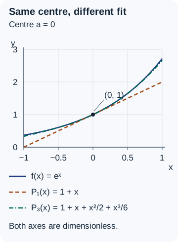
2. Turn the next derivative into an error bound

The remainder is the signed difference between the true function and the polynomial:

$R_n(x)=f(x)-P_n(x).$

A sufficient condition for the bound below is that $f$ has continuous derivatives through order $n+1$ on an open interval containing the whole segment from $a$ to $x$ . Choose a number $M\ge0$ such that

$|f^{(n+1)}(t)|\le M$

for every input $t$ between $a$ and $x$ , including the endpoints. The letter $t$ is a temporary input used to check that segment. Taylor’s theorem then gives

$|R_n(x)|\le\frac{M|x-a|^{n+1}}{(n+1)!}.$

Call the right-hand side $B$ . It is an upper bound, not usually the actual error. You do not need the smallest possible $M$ ; any justified upper bound works. The theorem and its hypotheses are reviewed in OpenStax’s section on Taylor approximation.

Build $P_n$ using derivatives at the centre.
Find the derivative of order $n+1$ and bound its magnitude on the entire segment.
Calculate $B$ and compare it with the allowed error $\varepsilon$ , a positive number.

If $B\le\varepsilon$ , the requested absolute accuracy is certified. If $B>\varepsilon$ , this bound is inconclusive: the approximation might still be accurate enough. Try a tighter derivative bound, a higher order, or a closer convenient centre.

3. Worked example: estimate a logarithm

Approximate $\ln(1.12)$ using order two at $a=1$

The natural logarithm $\ln x$ is defined for $x>0$ , and $\ln1=0$ . The centre 1 keeps the needed values simple:

$\begin{aligned}f'(t)&=1/t,\\f''(t)&=-1/t^2,\\f'''(t)&=2/t^3.\end{aligned}$

Thus $f'(1)=1$ and $f''(1)=-1$ . Build the polynomial before inserting the target input:

$P_2(x)=(x-1)-\frac{(x-1)^2}{2}.$

The displacement is $1.12-1=0.12$ , so

$\begin{aligned}P_2(1.12)&=0.12-\frac{0.12^2}{2}\\&=0.1128.\end{aligned}$

Check the error on the correct segment

On $[1,1.12]$ , all required derivatives are continuous. Since $t\ge1$ , the third derivative satisfies $0<2/t^3\le2$ . We can use $M=2$ :

$\begin{aligned}|R_2(1.12)|&\le\frac{2(0.12)^3}{3!}\\&=0.000576.\end{aligned}$

Result: $0.1128$ approximates $\ln(1.12)$ with absolute error at most $0.000576$ . In particular, it meets a tolerance of $0.001$ . This conclusion uses derivatives, not knowledge of the logarithm’s decimal value.

A later numerical check gives $\ln(1.12)\approx0.113328685$ , so the actual error is about $0.000528685$ , below the bound. That comparison illustrates the difference between an error and its upper bound; it is not the proof.

4. Worked example: meet a requested accuracy

Approximate $e^{0.2}$ with error at most $0.0005$

Use centre $a=0$ . Every derivative of $f(x)=e^x$ is $e^x$ , so every derivative at zero is 1. Here $e\approx2.718$ is the base of the natural exponential.

On $[0,0.2]$ , use the convenient bound $e^t\le e<3$ . Therefore $M=3$ works for every derivative order. It is deliberately generous, which makes it easy to justify without first calculating $e^{0.2}$ .

Try order two, then order three:

$\begin{aligned}B_2&=\frac{3(0.2)^3}{3!}=0.004,\\B_3&=\frac{3(0.2)^4}{4!}=0.0002.\end{aligned}$

The first bound does not certify the target. The second does. This is enough to choose order three; no claim about the best possible degree is needed.

$\begin{aligned}P_3(x)&=1+x+\frac{x^2}{2}\\&\quad+\frac{x^3}{6},\\P_3(0.2)&=\frac{458}{375}\\&=1.221333\ldots\end{aligned}$

Result: the exact polynomial value $458/375$ has absolute error at most $0.0002$ , safely below $0.0005$ . If you report the rounded value $1.22133$ , its rounding error is less than $0.000005$ . Adding that allowance still keeps the total error below $0.000205$ .

5. Avoid three false guarantees

“The derivative’s magnitude at the centre is my bound.” Only if that value bounds $|f^{(n+1)}(t)|$ everywhere between centre and target. Nor can you always check only the endpoints: an interior maximum is possible. Check where the derivative’s magnitude increases or decreases, use a known bound that applies throughout the interval, or justify another estimate.
“The first omitted term is always the error bound.” A Taylor coefficient uses a derivative at the centre. The bound above needs a derivative bound over a segment. For an alternating series, the magnitude of the first omitted term bounds the absolute error relative to the series sum when the omitted terms alternate, their magnitudes are nonincreasing, and they tend to zero. To use that rule for $f(x)$ , you must also know that the series sums to $f(x)$ .
“The curves look close, so the required accuracy holds.” A plot cannot certify a tiny numerical tolerance. Keep the interval, derivative bound and final error comparison in your written answer. If your final decimal is rounded, include that extra error too.

6. Four questions, from guided to independent

Try each question before opening its hint. An answer should include the centre, the polynomial, the segment used for $M$ , and the error conclusion.

1. Guided: a square root near a perfect square

Use the order-one Taylor polynomial of $f(x)=\sqrt{x}$ at $a=9$ to estimate $\sqrt{9.3}$ . Find a valid bound for the second derivative on $[9,9.3]$ . Is the absolute error at most $0.0005$ ?

Hint for question 1

Use $f(9)=3$ , $f'(9)=1/6$ , and $f''(t)=-1/(4t^{3/2})$ . Its magnitude decreases as $t$ increases through positive values.

Answer and reasoning for question 1

The linear polynomial and its value are

$\begin{aligned}P_1(x)&=3+\frac{x-9}{6},\\P_1(9.3)&=3.05.\end{aligned}$

The whole segment is positive. Its smallest input is 9, so $|f''(t)|\le1/108$ . Taking $M=1/108$ gives

$\begin{aligned}|R_1(9.3)|&\le\frac{(1/108)(0.3)^2}{2!}\\&=\frac1{2400}\\&\approx0.000416667.\end{aligned}$

Yes: $1/2400<0.0005$ , so the bound certifies the requested accuracy of the exact value $3.05$ .

2. Diagnose: the target moves to the other side

For $\ln(0.9)$ , a student reuses the order-two polynomial centred at 1 and gets $P_2(0.9)=-0.105$ . They reuse $M=2$ because $f'''(1)=2$ . What is wrong with that justification? Repair the bound.

Hint for question 2

The segment is now $[0.9,1]$ . Where does $2/t^3$ have its largest value on that segment?

Answer and reasoning for question 2

The polynomial value is correct, but the derivative bound is not. For inputs below 1, $2/t^3$ exceeds 2. Its maximum on this segment is at $t=0.9$ , so use

$M=\frac{2}{(0.9)^3}.$

All required derivatives remain continuous because the segment stays above zero. With distance $|0.9-1|=0.1$ ,

$\begin{aligned}|R_2(0.9)|&\le\frac{2(0.1)^3}{6(0.9)^3}\\&=\frac1{2187}\\&\approx0.000457247.\end{aligned}$

A later numerical check gives an actual error of about $0.000360516$ . That is below the repaired bound but above the student’s unjustified value $0.001/3$ . Moving the target can change $M$ , even when the polynomial stays the same.

3. Extend: a zero coefficient can help

Let $P(x)=1-x^2/2$ , and use $P(0.3)$ to approximate $\cos(0.3)$ . Show that $P$ , although it has degree two, is also the order-three Maclaurin polynomial for cosine. Use a fourth-derivative bound to certify absolute error at most $0.0004$ .

Hint for question 3

The first four derivatives of cosine are $-\sin x$ , $-\cos x$ , $\sin x$ , and $\cos x$ . The coefficient of $x^3$ is zero.

Answer and reasoning for question 3

At zero the function and first three derivatives are $1,0,-1,0$ . Consequently

$P_3(x)=1-\frac{x^2}{2},$

which has degree two. On $[0,0.3]$ , the fourth derivative is cosine and its magnitude is at most 1. Thus

$\begin{aligned}|R_3(0.3)|&\le\frac{(0.3)^4}{4!}\\&=0.0003375\\<0.0004.\end{aligned}$

The value $P_3(0.3)=0.955$ meets the target. We used order three in the theorem even though no cubic term appears. Order describes the derivatives matched, not necessarily the highest nonzero power.

4. Independent: one approximation over a whole interval

Approximate $e^x$ for every $x$ in $[-0.4,0.4]$ , using Maclaurin polynomials and the bound $M=3$ . Compare orders three and four. Which one does this bound certify for absolute error at most $0.001$ throughout the interval? State the chosen polynomial.

Hint for question 4

Every segment from 0 to an allowed target lies inside $[-0.4,0.4]$ , where $e^t<3$ . The greatest distance from the centre is 0.4. Use that distance in each bound.

Answer and reasoning for question 4

The derivative bound applies across the entire interval, and $|x|\le0.4$ . Therefore the following bounds hold for every allowed target:

$\begin{aligned}B_3&=\frac{3(0.4)^4}{4!}=0.0032,\\B_4&=\frac{3(0.4)^5}{5!}=0.000256.\end{aligned}$

Order four is certified; the order-three bound is inconclusive. Use

$\begin{aligned}P_4(x)&=1+x+\frac{x^2}{2}\\&\quad+\frac{x^3}{6}+\frac{x^4}{24}.\end{aligned}$

The absolute error is at most $0.000256$ everywhere on the stated interval. This is a single guarantee for many inputs, rather than a calculation for just one input.

7. Check your method and choose a next step

Can you explain why your centre is convenient, why your $M$ covers every input between centre and target, and whether your final bound meets the requested tolerance? If one answer is missing, fix that step before adding more terms.

Try the Taylor error check on the McGill MATH 262 page to compare a certified approximation with one whose error exceeds the tolerance.

If your difficulty is deciding whether an infinite sum converges, revisit three convergence decisions to explain. If it is finding all inputs that make a power series converge, continue with intervals and endpoint tests. Those questions do not replace the finite-error check taught here.

Course context: Concordia’s official MATH 205 description includes Taylor and Maclaurin series. These are original study examples, not course assessments. Your current course outline determines the methods and scope required in your class.

Useful for

Work on the step you’re missing.

Tell us the subject and your preferred time. Nablio confirms the details by text or email.

Request a lesson