Conditional Probability and Bayes: Choose the Right Denominator

1. Start with the group you are choosing from

A hypothetical lot contains 1,000 components: 40 are defective and 960 are sound. An inspection flags 36 of the defective components and 48 of the sound components. The other 4 defective and 912 sound components are not flagged.

Choose one component uniformly at random: each of the 1,000 components has the same chance of selection. You learn that it was flagged. What is the probability that it is defective?

The denominator tells you which group you are considering. Using 1,000 would answer a different question: how often a uniformly selected component is both defective and flagged.

2. Define the events and read the notation

An outcome is the component selected. An event is a set of outcomes with a stated property. Let $D$ be the event “the selected component is defective” and $F$ the event “the selected component is flagged.” The complement $D^c$ means “not defective,” which is “sound” in this model; $F^c$ means “not flagged.” These classifications are exhaustive: every component is in exactly one defect category and exactly one flag category.

The symbol $P$ denotes probability. For this uniform selection from a finite lot, an event’s probability is its count divided by the lot’s size. Thus $P(D)=40/1000=0.04$.

The intersection $D\cap F$, read “$D$ and $F$,” requires both properties. The conditional probability $P(D\mid F)$, read “probability of $D$ given $F$,” restricts attention to outcomes in $F$. The event after the vertical bar sets the denominator. This definition requires that the conditioning event have positive probability.

3. Read the frequency tree, then regroup

The tree first splits the lot by defect status, then by inspection result. Read a path as a sequence of classifications of the same selected component. The four terminal counts add to 1,000. Branch lengths carry no numerical meaning.

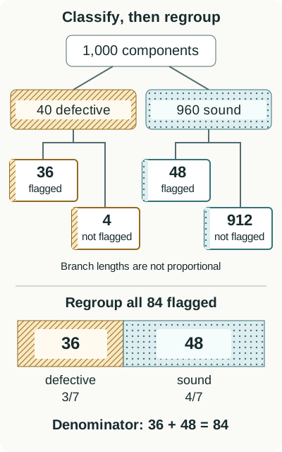
Text equivalent: Of 1,000 components, 40 are defective: 36 flagged and 4 not flagged. The other 960 are sound: 48 flagged and 912 not flagged. Regrouping the flagged components gives 84 in total: 36 defective and 48 sound. The bar allocates $3/7$ of its width to defective components and $4/7$ to sound components. Diagonal stripes mark defective components; dots mark sound components.

The flagged group contains more sound components than defective ones. A small flag rate among the much larger sound group can still contribute many flagged components. The original proportion of defective components is the base rate, here 4%. Ignoring it would miss why the much larger sound group contributes 48 of the 84 flags, despite its lower flag rate.

4. Build the multiplication and total-probability rules

Introduce general events $A$ and $B$ in the same sample space, the set of all possible outcomes. Conditional probability divides the probability of their intersection by the probability of the conditioning event:

Multiply both sides by $P(B)$. This gives a multiplication rule. It does not require independence.

Apply the rule to the defective branch. The probability of entering that branch is $40/1000$. Within that branch, the fraction flagged is $36/40$. Multiplying cancels the intermediate group size:

To find the probability of being flagged, add the flagged defective and flagged sound branches. These groups are disjoint, meaning no component is in both; together they contain every flagged component. The events $D$ and $D^c$ form a partition: non-overlapping groups covering the whole sample space.

Here the conditional flag rate among sound components is $P(F\mid D^c)=48/960=0.05$. Weight each conditional rate by the proportion of the lot in its group:

Simply adding 90% and 5%, or averaging them equally, would ignore the very different group sizes.

5. Derive Bayes’ formula and interpret the result

Return to the question “defective given flagged.” The numerator is the probability of both properties. The denominator includes every way a component can be flagged. Use the multiplication rule for the numerator; keep the total flag probability calculated from the partition in Section 4 as the denominator:

Here $P(F)$ is the total flag probability: add the flagged-defective and flagged-sound contributions, as in Section 4.

This is Bayes’ formula for these two defect categories, with $P(F)>0$. In this version both defect categories also have positive probability, so the conditional flag rates used in Section 4 are defined. The prior probability $P(D)$ is the probability of a defect before learning the flag result. The posterior probability $P(D\mid F)$ is the probability after learning that result. Here “before” and “after” describe available information, not a change in the component.

The flag raises the probability of a defect from 4% to about 42.9%. It provides useful information without guaranteeing a defect. The fraction is the same $36/84$ we found by counting; Bayes’ formula organizes that reasoning when probabilities are given instead of counts.

Check the denominator. Dividing by 0.04 would condition on a defect. Dividing by 0.084 conditions on a flag. Name the known event in words before choosing either.

6. Distinguish independence from disjointness

Two events are independent when their joint probability equals the product of their individual probabilities. When the conditioning event has positive probability, this is equivalent to saying that learning it does not change the other event’s probability.

To test independence, ask whether this equality holds:

In this lot, the left side is 0.036. The product on the right is $(0.04)(0.084)=0.00336$. They are unequal, so defect status and flag status are dependent. Equivalently, $P(D\mid F)=3/7$ differs from $P(D)=0.04$.

Disjoint events cannot occur together. Independent events do not change one another’s probabilities. Here $D$ and $F$ are not disjoint, because 36 components have both properties, and they are not independent. By contrast, $D$ and $D^c$ are disjoint. Since both have positive probability, they are not independent either: learning one rules out the other.

7. Practise choosing the denominator

For each question, write the relevant group in words before calculating. Try it unaided, open a hint if needed, then compare your reasoning with the answer. The questions move from reading a condition to changing the information, changing the base rate and checking an assumption.

Take this habit to your next problem: identify the possible outcomes, name the known event, count or calculate every route into that event, then divide the relevant joint probability by its probability. Check that your answer lies between 0 and 1 and explain which group it describes.

8. Connect the ideas to your course

For Concordia MAST 221, use this lesson to practise conditional probability: distinguish the two conditional directions and explain the denominator before using Bayes’ formula. For STAT 249, focus first on the probability foundations: events, complements, intersections and the choice of reference group.

McGill’s current Mathematics and Statistics course listing includes conditional probability, Bayes’ theorem and independence in MATH 323. Work through the derivation and the independence check, then compare the notation with your current course outline. Use that outline to decide which topics and methods to practise for your section.

For your next study session, bring one problem and mark the event you are given. Explain which outcomes remain possible and why they form your denominator.

These examples practise one group of probability skills; they do not cover the full content of any course listed here. The official descriptions below establish topic connections, while your current course outline sets the scope for your section.

• Concordia: Mathematics and Statistics course descriptions
• McGill: Mathematics and Statistics course listing — MATH 323