Conditional Probability and Bayes: Choose the Right Denominator
Start with counts, distinguish “given” from “and,” derive Bayes’ formula and test independence with a frequency tree and four explained exercises.
Calculus-based probability, with original practice on conditional densities and sample means.
MATH 323 at McGill develops probability using differential and integral calculus. It moves from events and counting to discrete and continuous distributions, independence, probability inequalities and limit theorems. McGill lists Fall 2026 and Winter 2027 offerings. The practice below focuses on conditional densities and the variability of a sample mean.
Review definite integrals, inequalities, expectation and variance. The short check below asks what averaging independent observations changes. The worked example then uses an iterated integral to normalize a joint density before conditioning.
McGill lists MATH 141 or equivalent as the prerequisite. The course is intended for students in Science, Engineering and related fields with differential and integral calculus, and is not open to students who have taken or are taking MATH 356. Confirm your eligibility with McGill.
Check the official course catalogueLet be independent, identically distributed real random variables, with common mean and finite variance . Here is the sample size and labels an observation. Define the sample mean by A student says: “Going from 25 to 100 observations halves the variance, and the weak law of large numbers guarantees that the mean equals at 100 observations.” Correct both claims. What happens to the standard deviation?
For a real constant , . Independence lets you add the variances of these observations. Standard deviation is the square root of variance. Does a statement about a probability tending to zero force an error to be exactly zero at a fixed sample size?
Write for variance. Independence gives Dividing each observation by contributes , not , before the variances are added.
The variance changes from to : it is divided by four. With the common standard deviation, the sample mean’s standard deviation is . It changes from to , so it is halved.
For any fixed tolerance , Chebyshev’s inequality gives The bound tends to zero as grows. Under the stated assumptions, this proves the weak law of large numbers: the probability of an error at least as large as the fixed tolerance tends to zero. It does not guarantee exact equality at , or at any other fixed sample size.
The check above finds the spread of an average. The central limit theorem (CLT) adds a limiting distribution that can help approximate probabilities.
Revisit the sample-mean variance check
Let be independent, identically distributed observations with common mean and finite, positive variance . The positive integer is the sample size, labels an observation, and is the population standard deviation. The random quantity here is the sample mean , not one observation. Its standard deviation, also called its standard error, is .
Define the dimensionless standardized mean by Under these assumptions, the CLT says that the distribution of approaches the standard normal distribution as grows. Write for a standard normal variable, with mean zero and variance one, and for its cumulative probability at a dimensionless cutoff .
For a nonnormal population, a finite-sample normal calculation is an approximation. Its accuracy depends on the population’s shape, sample size and event, especially in the tails. There is no universal “” guarantee. If the independent observations instead have a common normal distribution, their sample mean is exactly normal for every , and is exactly standard normal.
The weak law says that, for each fixed tolerance , the probability tends to zero. The tolerance has the same units as an observation. The CLT describes the limiting shape of the standardized fluctuations . The weak law alone supplies neither a normal approximation nor an exact finite-sample probability.
Use this hypothetical model: each duration is uniform between 0 and 12 minutes, and the durations are independent. All , , and are measured in minutes; variance is in squared minutes. Thus , and . For , approximate : the chance the average exceeds 6.5 minutes.
The population is bounded and symmetric, with finite variance, so this is a reasonable practice setting for a CLT approximation. The individual durations are uniform, not normal; the answer must still be labelled approximate.
For 48 independent observations, the standard error is minutes. The population standard deviation measures the spread of an individual duration; use the standard error for this average.
The threshold is The numerator and denominator both have units of minutes, so has no units. The desired event becomes .
From a standard normal table or calculator, Under this model, about 15.9% of independent samples of 48 durations have an average above 6.5 minutes. This is a statement about repeated sample means, not the percentage of individual durations above 6.5 minutes.
Keep the same independent uniform-duration model and the same 6.5-minute threshold, but take . Find the new standard error, the standardized cutoff and the CLT approximation to . Explain why the probability changes.
Quadrupling halves the standard error: minutes. The dimensionless cutoff is . Therefore The chance is now about 2.3%. The threshold is two standard errors above the unchanged mean instead of one, so fewer sample means exceed it. Neither finite-sample distribution is exactly normal.
A student claims that makes any average exactly normal. In one dataset, every observation repeats the same single duration drawn from the uniform model; in another, the observations are independent with a common distribution but infinite variance. Can the iid, finite-variance CLT stated above justify either claim? Here “iid” means independent and identically distributed.
No. Repeating one random duration creates dependent observations. Their average equals that one duration, so averaging does not reduce its spread. The formula cannot be used here.
Infinite variance violates a hypothesis of this version of the CLT, so it does not justify the displayed standardization or a normal approximation. Other limit theorems require their own assumptions. Even with iid observations and finite positive variance, alone proves neither exact normality nor a specified approximation accuracy.
Original selected-topic practice, not an official McGill assessment or a complete MATH 323 review. Use your section’s current outline to confirm the methods expected.
A transformation changes the values a random variable can take, but probabilities still come from the original model. Start with the event , not a memorized density formula. This lesson develops the cumulative distribution function (CDF) method, including the nonmonotone transformation .
Prerequisites: integrals of one-variable densities, inequalities, inverse functions and the chain rule. All numerical models below use dimensionless variables. The examples and exercises are original practice, not official assessment questions.
Let have density on a set , and define . First find the range of on . A positive input need not produce a positive output; a nonlinear function can turn around inside the support. Include boundary values when describing the closure of the support, even when their individual probabilities are zero.
For any real cutoff , the CDF is Define the input set . Then The set may be empty, one interval, several intervals or all of . A sketch of helps, but the inequality and support intersection determine the actual integration limits.
For cutoffs below the output range, the CDF is zero; at or above its greatest value, if one exists, the CDF is one. Within the range, locate every cutoff where an inverse branch meets an endpoint of . These are possible breakpoints of the formula. Check that is nondecreasing and right-continuous, with limits zero and one at the two infinities.
On smooth portions of an absolutely continuous distribution, . If is strictly monotone and differentiable, its inverse is differentiable, and is nonzero on the relevant interval, then The absolute value keeps the density nonnegative. This expression is zero outside the transformed support.
For finitely many smooth monotone branches, add the contributions from every inverse value that lies in the input support: Use this only away from critical values where the displayed denominators vanish. A density may be unbounded near such a value and still integrate to one. The CDF method remains the safer starting point.
A continuous input does not guarantee a continuous output distribution. If maps an interval of positive input probability to one value , then . The CDF jumps at ; ordinary differentiation misses that mass. A fully correct answer must state any point masses as well as the continuous part. Exercise 4 makes this distinction explicit.
For a continuous and a strictly decreasing , at an interior output value, The event is , not . Continuity of is why including the endpoint does not change this probability. With atoms, the correct complement uses the left limit of .
For , Intersect this interval with the input support. Keeping only loses the negative branch; keeping both branches after one has left the support counts nonexistent outcomes.
Let for , and zero elsewhere. Define . Find the CDF and density of , then compute .
The input density integrates to , and for . The function decreases from arbitrarily large positive values toward zero. Thus almost surely, with support closure .
For , . For , Therefore At , this formula gives zero, consistent with no atom at zero.
The density is for , and zero for . Its value at the single point zero may be chosen arbitrarily. The normalization is . As an independent check, the inverse gives .
Equivalently, means , whose probability is . Larger values of the transformed variable correspond to smaller, not larger, input values.
Let be uniform on , so inside this interval. Define . Find its CDF and density, and calculate .
The transformed support is , not : the input interval contains zero. For , both and lie in . For , the negative inverse lies below , so the event begins at the support endpoint .
For , the event is , an interval of length . For , it is , an interval of length . Divide each length by the total input length 3:
Values at the isolated points 0, 1 and 4 do not affect integrals. Below 1, two inverse branches contribute each; above 1, only the positive branch contributes. A single formula that retains both branches all the way to 4 would overcount.
Both CDF pieces give at 1, and the upper piece tends to one at 4. There is no CDF jump, hence no point mass at the breakpoint. The density is unbounded near zero, but
Finally, Directly, the admissible input interval is . The corresponding negative interval lies entirely outside the input support; the endpoint is excluded by the strict inequality .
Try each problem before revealing the solution. For every CDF, give its values outside the transformed range as well as inside it.
Let and . Find the support, CDF and density of . Compute .
The increasing map sends to . For , is , so The CDF is zero below and one above 7.
for , and zero outside; its integral is . Thus . Equivalently, the input event is , an interval of length 2 out of 4.
Let and . Find its CDF and density. Compute and explain the inequality direction.
The output support is . For , is equivalent to , since both variables here are positive. Hence The CDF is zero below and one above 1; its endpoint values agree with these outer pieces.
The density is for , and zero outside. Its integral is . At , the CDF is , exactly . Using would select the wrong tail.
Let for , and zero elsewhere. Put . Find its CDF and density, then compute . Why can you not use twice the positive-branch contribution?
The input density is nonnegative and integrates to one. The output support is . For , The odd term cancels over the symmetric interval. The CDF is zero below zero and one above one.
Differentiation gives on , zero outside. Its integral is one. The branch formula gives the same result:
The two input density values are and , so their contributions are not equal. Doubling the positive branch would produce the incorrect density , whose integral is , not one.
Directly from the input, : the cubic term integrates to zero. These checks agree because .
Let and . Find the full CDF, identify any point mass and the continuous part, and compute and . Explain why differentiating the CDF alone does not describe the entire law.
Every input maps to zero, so . The output support is . For , the event is , including all negative input values. Therefore
The CDF jumps from zero to at zero. The continuous part has density on , contributing total probability . Together the atom and continuous part total one. There is no ordinary density with respect to length that represents the entire distribution: integrating the derivative only gives .
The mean is The atom contributes to probabilities but contributes zero to this expectation because its location is zero.
Original selected-topic enrichment for probability study alongside MATH 323. This is not an official McGill assessment, a current-term syllabus claim or a complete course review. Check your section’s current outline for the methods expected.
Let and be dimensionless continuous random variables. Their joint density is on the region and zero elsewhere. Here are real coordinates and is an unknown constant. Let be the event . Find , then using a conditional density.
At each fixed between 0 and 1, the horizontal slice runs from to . The density is nonnegative and its total integral must be 1: First, . Then Therefore . The triangle specifies where the density can be positive; its area alone is not the probability calculation.
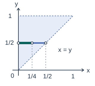
The marginal density describes alone. For , find it by integrating over all allowed values of : It is zero elsewhere. Check that . At the chosen value of Y, .
For , the conditional density is the joint density divided by the positive marginal density. For , It is zero for all other . This is normalized because Here ; conditioning is defined by the density formula, not by dividing probabilities that a continuous variable takes an exact value.
Setting gives density for , and zero elsewhere. The event restricts the integral to : The left half of the allowed interval carries only one quarter of the conditional probability: the density increases with , so the conditional distribution on that interval is not uniform.
With the same conditioning value , find Should you extend the formula all the way to ?
No. The conditional density is only on , and zero elsewhere. Every allowed value already satisfies , so the probability is . Using the formula outside the interval where the density can be positive would give , which is not a probability.
If the bounds were the hard part, review horizontal and vertical slices before doing more probability calculations. If normalization was the hard part, check the total integral at each stage: joint, marginal and conditional.
For the bounds in this density example, revisit horizontal and vertical slices in the existing double-integral guide. Its later polar-coordinate exercises are separate calculus practice. Review how to read integration slices
Bring a MATH 323 problem you’re stuck on or a probability concept you’d like to understand better. We can also start with the basics and build your confidence step by step. If you have a course outline, you can share it to help choose the topics to work on. A tutor can help translate the statement into events or random variables, sketch the support, set the integration bounds and check each normalization step. For averages and limit theorems, a tutor can trace the variance calculation and test whether the assumptions justify your conclusion.
Practise defining the events or random variables before choosing a formula. For densities, mark the support and check normalization; for a limit theorem, state the assumptions and the quantity that converges. These exercises target selected skills. Your section’s current instructions determine the material and methods for each assessment.
We work through permitted practice and comparable problems, without completing graded assignments or exams on your behalf.
The Bayes guide reviews conditioning on an event of positive probability. The worked example here uses a density when conditioning on a continuous value. Review conditioning on events before conditional densities
Start with counts, distinguish “given” from “and,” derive Bayes’ formula and test independence with a frequency tree and four explained exercises.
Send your topic and preferred times. We’ll confirm tutoring coverage and the schedule by text or email before payment.
Nablio is an independent service and is not affiliated with this institution.