Stuck on a step? Text us Email us Request a lesson
A fitted line is a starting point for checking a model
A sensor’s output rises as the applied load increases. Can a straight line describe that relationship usefully? You will fit a line, compare its predictions with the observations, then examine a changed dataset that looks strongly associated but leaves a curved residual pattern.
Start once you can substitute into a line equation and calculate a mean. For slope, intercepts and reading coordinates, use Points, Slope and Straight-Line Graphs. You do not need calculus for the calculations here.
Define the quantities before calculating
In this invented teaching example, a technician applies six known loads to a sensor. The data are constructed for this lesson; they are not measurements from a real device, an experiment or a manufacturer’s specification.
- Explanatory variable: x is applied load, measured in newtons (N).
- Response variable: y is observed sensor output, measured in millivolts (mV).
- Fitted value: ŷ, read “y-hat”, is the output predicted by the fitted line at a specified x. It also has units of mV.
- Residual: e is observed output minus fitted output, so , in mV.
| Applied load x (N) | Observed output y (mV) |
|---|---|
| 0 | 1.1 |
| 1 | 2.8 |
| 2 | 5.1 |
| 3 | 7.1 |
| 4 | 8.8 |
| 5 | 11.1 |
The observations form six pairs; keep each load with its own output. The points rise and look close to a straight line. That makes a straight-line model worth examining, but the appearance alone does not settle whether it is adequate.
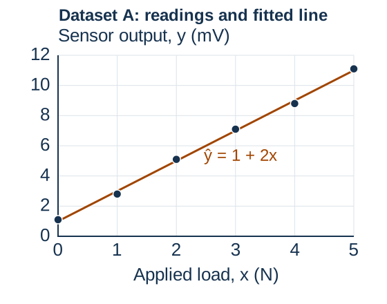
What are we assuming?
For this exercise, treat the loads as known accurately compared with the output variation, give all six readings equal weight, and allow a fitted intercept. We are predicting output from load. Estimating an unknown load from an output is a separate calibration question; reversing the labels does not automatically give the same regression.
The least-squares calculation itself does not require normally distributed data. To use a line beyond a description of these six points, we would need evidence that a straight-line relationship is reasonable over the intended range and that the measurement conditions remain comparable. The data alone do not establish independent errors or constant variability. Six readings cannot establish a device’s performance or the accuracy of future predictions.
Fit the line using every observation
Write the fitted line as , where a is the fitted intercept and b is the fitted slope. These letters have different roles from any notation you may have used for a line through two exact points.
A line through the first and last observations is one possible line. Least squares instead chooses a and b to make the sum of squared vertical residuals as small as possible:
Here n is the number of observations, i labels one observation, and Σ means add over all observations. Squaring prevents positive and negative residuals from cancelling. It also makes a large residual count more heavily. These are vertical output differences, not the shortest perpendicular distances to the line. SSE has units of mV².
Step 1: find the two means
There are n = 6 observations. The loads sum to 15 N and the outputs sum to 36 mV. A bar denotes a mean:
Step 2: measure variation around the means
Define and . The first measures the spread of the inputs; the second combines the paired input and output deviations.
| x (N) | x − x̄ (N) | y − ȳ (mV) | (x − x̄)² (N²) | (x − x̄)(y − ȳ) (N·mV) |
|---|---|---|---|---|
| 0 | −2.5 | −4.9 | 6.25 | 12.25 |
| 1 | −1.5 | −3.2 | 2.25 | 4.80 |
| 2 | −0.5 | −0.9 | 0.25 | 0.45 |
| 3 | 0.5 | 1.1 | 0.25 | 0.55 |
| 4 | 1.5 | 2.8 | 2.25 | 4.20 |
| 5 | 2.5 | 5.1 | 6.25 | 12.75 |
| Total | 0 | 0 | 17.50 | 35.00 |
For example, at x = 1 N, the product is (−1.5)(−3.2) = 4.80 N·mV. Keep each pair together: multiplying a deviation from one row by an output deviation from another row changes the fit.
Step 3: calculate slope and intercept
For an ordinary, equally weighted least-squares fit with an intercept, provided the x values are not all the same,
The units work: (N·mV)/N² = mV/N. Multiplying the slope by a load in N gives an output in mV, which can be added to the intercept.
Keep this unit convention whenever you use the numerical equation. The slope says that the fitted output increases by 2 mV for an additional 1 N of load. It does not say that every observed reading increases by exactly 2 mV. The intercept is the predicted output at zero applied load, 1 mV. Zero lies in our observed range, so this interpretation does not require extrapolation. The actual reading there was 1.1 mV.
Step 4: check a property of the fitted line
At the mean load, the prediction is 1 + 2(2.5) = 6 mV, the mean output. A least-squares line with an intercept passes through (x̄, ȳ). This catches some arithmetic mistakes; it is not evidence that a straight line is the right model.
If all input values were identical, Sxx would be zero and this slope formula would be undefined: the data would not show how the output changes with the input. Keep several distinct input values, and do not confuse the number of readings with the range they cover.
Use residuals to see what the line misses
Calculate each fitted value from the line, then subtract in the same order every time: observed minus predicted.
| x (N) | Observed y (mV) | Predicted ŷ (mV) | Residual e (mV) |
|---|---|---|---|
| 0 | 1.1 | 1.0 | +0.1 |
| 1 | 2.8 | 3.0 | −0.2 |
| 2 | 5.1 | 5.0 | +0.1 |
| 3 | 7.1 | 7.0 | +0.1 |
| 4 | 8.8 | 9.0 | −0.2 |
| 5 | 11.1 | 11.0 | +0.1 |
At x = 1 N, ŷ = 1 + 2(1) = 3 mV, so e = 2.8 − 3 = −0.2 mV. The point lies below the line: the line overpredicts the observed output by 0.2 mV. At x = 2 N, e = 5.1 − 5 = +0.1 mV; the point lies above the line and the line underpredicts by 0.1 mV.
A residual plot keeps x on the horizontal axis but replaces y with e on the vertical axis. The sloping fitted line becomes the horizontal reference e = 0. Do not join the residual dots: each is a separate observation.
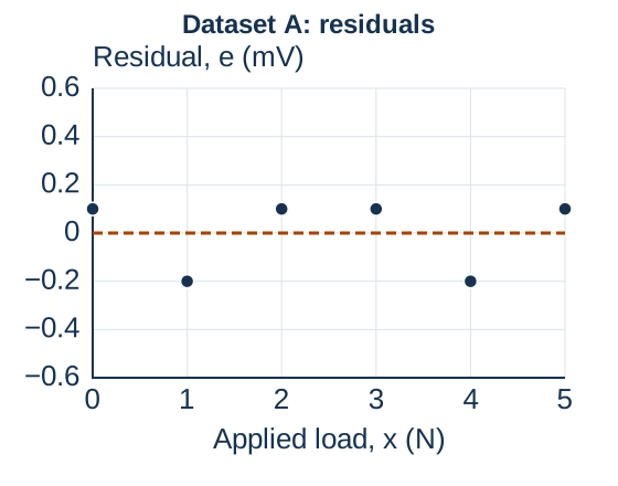
Here the discrepancies are at most 0.2 mV, with no clear U-shaped pattern at these six loads. That is a limited description, not a declaration of random errors or an accurate device. Whether 0.2 mV is small enough depends on the purpose and tolerance of a real application, neither of which this invented example specifies.
A zero sum is an arithmetic check, not a certificate
The residual sum is 0.1 − 0.2 + 0.1 + 0.1 − 0.2 + 0.1 = 0 mV. The squared residual sum is 4(0.1²) + 2(0.2²) = 0.12 mV².
With an intercept, an ordinary equally weighted least-squares fit has and , apart from rounding. These are properties of the fitting method even when a straight line is inadequate. They do not mean every residual is zero, and they do not require equal numbers of positive and negative residuals. The same statements need not hold for a line forced through the origin or for arbitrary chosen coefficients.
Change the data: high correlation can hide curvature
Now replace the outputs with dataset B, another deliberately invented set, at the same loads. This is a comparison of two teaching datasets, not a claim about a sensor changing over time.
| x (N) | Observed y (mV) | Predicted ŷ (mV) | Residual e (mV) |
|---|---|---|---|
| 0 | 1.5 | 1.0 | +0.5 |
| 1 | 2.9 | 3.0 | −0.1 |
| 2 | 4.6 | 5.0 | −0.4 |
| 3 | 6.6 | 7.0 | −0.4 |
| 4 | 8.9 | 9.0 | −0.1 |
| 5 | 11.5 | 11.0 | +0.5 |
The means are still x̄ = 2.5 N and ȳ = 6 mV. Sxx is still 17.5 N². The six centred products now add to 13.75 + 4.65 + 0.70 + 0.30 + 4.35 + 13.75 = 35 N·mV. Thus the least-squares fit is again ŷ = 1 + 2x. We refitted the changed data; we did not merely assume the old coefficients still apply.
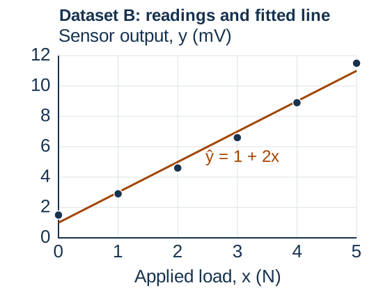
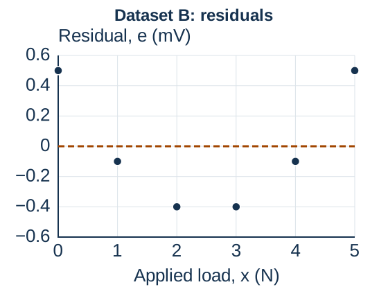
The residuals are positive at the ends and negative through the middle. This systematic U-shaped pattern is a reason to question the straight-line form. Rechecking measurements, examining the measurement conditions and collecting more observations could help determine whether a different model is justified. Six constructed points do not establish the true physical relationship or identify a unique replacement model.
Check the high-correlation claim
The correlation coefficient r is a unitless measure of linear association. For nonconstant x and y values, define ; then .
For dataset B, the output deviations are −4.5, −3.1, −1.4, 0.6, 2.9 and 5.5 mV. Their squares add to 70.84 mV², so
This is very close to +1 even though the residuals curve. For this ordinary single-predictor fit with an intercept, R² = r² ≈ 0.988. This says the line accounts for about 98.8% of the observed variation around the mean in this dataset. It is not a 98.8% probability that the line is correct, or a promise about future readings.
Dataset B also has zero residual sum, yet its squared residual sum is 2(0.5²) + 2(0.1²) + 2(0.4²) = 0.84 mV². Neither a zero sum nor high correlation replaces a look at the pattern.
Keep the conclusion proportional to the evidence
- A curved residual pattern suggests the line is leaving a systematic feature unexplained.
- A plot without obvious curvature does not prove a model correct. Small samples can hide patterns, and a plot against x alone cannot establish independence or other measurement assumptions.
- A widening residual spread would raise a different question about variability. One unusually large residual would call for investigation; it would not justify deleting the observation automatically.
- Interpolation uses an input within the observed range. Extrapolation goes outside it, where these observations provide no direct check of the line.
- A fitted association, even with a tidy residual plot, does not by itself establish cause and effect.
Five questions: calculate, interpret, then challenge the model
These questions are original practice. Open a hint when useful, compare your reasoning with the full solution, then try the changed version. A calculator can help with arithmetic; explain what each result means.
1. Fit a new calibration line
A separate invented sensor dataset has loads x = 0, 1, 2, 3 N and outputs y = 1, 3, 4, 6 mV, paired in order. Find the equally weighted least-squares line with an intercept. Interpret its slope and zero-load prediction.
Hint for question 1
Find both means, then calculate Sxx and Sxy. The slope is Sxy/Sxx, not the mean of the y values and not necessarily the slope through the endpoints.
Full solution for question 1
The means are x̄ = 1.5 N and ȳ = 3.5 mV. The x deviations are −1.5, −0.5, 0.5, 1.5 N; the y deviations are −2.5, −0.5, 0.5, 2.5 mV.
Sxx = 2.25 + 0.25 + 0.25 + 2.25 = 5 N². Sxy = 3.75 + 0.25 + 0.25 + 3.75 = 8 N·mV. Thus b = 8/5 = 1.6 mV/N and a = 3.5 − 1.6(1.5) = 1.1 mV.
The fit is ŷ = 1.1 + 1.6x, with x in N and ŷ in mV. Each additional newton raises the fitted output by 1.6 mV; the predicted zero-load output is 1.1 mV. At x̄ = 1.5 N, the line gives 3.5 mV as required.
Predicted outputs are 1.1, 2.7, 4.3 and 5.9 mV; residuals are −0.1, +0.3, −0.3 and +0.1 mV. Their sum is zero. The endpoint slope, (6 − 1)/(3 − 0) = 5/3 mV/N, is different because it ignores the two middle observations when choosing the line.
Retry: change the outputs
Keep x = 0, 1, 2, 3 N, but use y = 2, 3, 5, 6 mV. Find the new line and check its prediction at the mean load.
Retry solution for question 1
Now ȳ = 4 mV, while x̄ = 1.5 N and Sxx = 5 N². The y deviations are −2, −1, 1, 2 mV, so Sxy = 3 + 0.5 + 0.5 + 3 = 7 N·mV. Hence b = 1.4 mV/N and a = 4 − 1.4(1.5) = 1.9 mV.
The line is ŷ = 1.9 + 1.4x. At x = 1.5 N it predicts 4 mV. Its predictions are 1.9, 3.3, 4.7, 6.1 mV; residuals are +0.1, −0.3, +0.3, −0.1 mV, again summing to zero.
2. Read a residual’s sign
Return to dataset A’s line ŷ = 1 + 2x. At x = 4 N, the observed output is 8.8 mV. Calculate the prediction and residual. Does the line overpredict or underpredict, and where is the observation relative to the line?
Hint for question 2
Substitute the load first. Then calculate observed minus predicted. A positive residual belongs above the line.
Full solution for question 2
ŷ = 1 + 2(4) = 9 mV. The residual is e = 8.8 − 9 = −0.2 mV. The observation is below the line, and the line overpredicts by 0.2 mV. Saying “−0.2 N” would give the input’s unit to an output discrepancy; saying “underpredicts” would reverse the comparison.
Retry: a new check reading
Keep the same fitted line without refitting it. A new reading at x = 3 N gives y = 7.3 mV. Find the residual and explain its sign.
Retry solution for question 2
The prediction remains ŷ = 1 + 2(3) = 7 mV. The difference is 7.3 − 7 = +0.3 mV: the new point lies above the line, which underpredicts this reading by 0.3 mV. This new reading was not used to fit the line, so the original fitted-data residual-sum property does not require this additional difference to sum to zero with the old residuals.
3. Separate interpolation from extrapolation
Dataset A covers loads from 0 to 5 N. Using its fitted line, predict the output at 2.5 N and at 6 N. Classify each calculation and state what the numbers do not guarantee.
Hint for question 3
The classification depends on the input range, not whether the predicted output is positive or close to an observation.
Full solution for question 3
At 2.5 N, ŷ = 1 + 2(2.5) = 6 mV. This is interpolation because 2.5 lies within [0, 5]. At 6 N, ŷ = 1 + 2(6) = 13 mV. This is extrapolation because 6 exceeds the largest observed load.
Both substitutions are valid arithmetic. The extrapolation assumes the line remains useful beyond the measured range, which these data do not check. Even the interpolated value is a model prediction, not an observed reading or a guarantee that a future output will equal 6 mV.
Retry: check two other loads
Calculate the predictions at 4.5 N and 7 N. Would the fact that the residuals at the six fitted loads are small make both predictions equally supported?
Retry solution for question 3
The predictions are 10 mV at 4.5 N and 15 mV at 7 N. The first is interpolation; the second is extrapolation. Small discrepancies within 0–5 N give no direct evidence about behaviour at 7 N. They also do not quantify the uncertainty of either prediction. New observations in the intended range would be useful before relying on the extension.
4. Challenge the model, not the subtraction
A student approves dataset B’s line because r ≈ 0.994 and the residuals sum to zero. Use the residual pattern to explain what this argument misses. Identify where the line overpredicts and underpredicts.
Hint for question 4
Read the residuals from left to right: +0.5, −0.1, −0.4, −0.4, −0.1, +0.5 mV. Ask whether the signs and sizes depend systematically on the load.
Full solution for question 4
The line underpredicts at 0 and 5 N, where the residuals are positive. It overpredicts at 1, 2, 3 and 4 N, where they are negative, with the largest overpredictions in the middle. The U-shaped pattern suggests that the straight-line form misses systematic curvature.
High r summarizes the strong overall linear association; it does not rule out this pattern. Zero residual sum follows from the equally weighted least-squares fit with an intercept, even for an inadequate line. A reasonable next step is to check the readings and conditions and collect more data before choosing another model. The plot does not prove a quadratic law or establish future accuracy.
Retry: a smaller dataset
For another fitted line with an intercept, residuals at x = 0, 1, 2, 3 N are +0.2, −0.2, −0.2, +0.2 mV. A student says their zero sum proves the model is correct. What can you conclude?
Retry solution for question 4
The sum is indeed zero, but that is only consistent with the fitting method. Positive ends and negative middle suggest a possible curved pattern. With only four observations, its interpretation is especially uncertain. You can flag the pattern and seek more information; you cannot declare either that the line is correct or that a particular curved model is established.
5. Keep association separate from causation
In a separate invented observational study, a technician records room temperature and sensor output while the applied loads also vary. A positive regression slope relates temperature to output. Does it show that increasing room temperature causes the fitted increase in output? Explain why the applied load matters.
Hint for question 5
The two plotted variables are not the only things that changed. Think about a variable that can affect the output and also vary with the recorded temperature.
Full solution for question 5
No. The fitted slope describes an association in those observations. If higher loads happened to be used when the room was warmer, load could help explain the association between temperature and output. The regression alone cannot separate these explanations.
We would need information about how measurements were collected and how other conditions were controlled. A carefully designed experiment could help investigate a temperature effect. A strong correlation or a residual plot without an obvious pattern cannot, on its own, turn this observational comparison into a causal result.
Retry: change several things together
A technician replaces a sensor’s battery and changes the applied load at the same time. The next output is higher. Does a fitted line from earlier readings show that the new battery caused the increase?
Retry solution for question 5
No. Both the battery condition and the load changed. A line describing earlier data does not identify which change caused this difference. Comparable measurements with the load controlled would help investigate the battery’s effect; the single before-and-after comparison does not isolate it.
Choose the next step from the difficulty
- If slope and intercept are unclear, revisit the straight-line foundation, then question 1.
- If residual signs are getting reversed, write “observed − predicted” before every subtraction and repeat question 2.
- If a numerical answer feels more certain than the evidence, revisit questions 3–5 and state the input range, residual pattern and limits in words.
Is this the whole regression topic for my course?
No. This is selected practice in fitting and checking a single-predictor straight-line model. Compare it with your current section’s outline and instructions. It does not cover formal inference, prediction intervals, multiple regression or process-control charts, and it makes no claim about a particular examination.
Can I ask for help before I have an attempted solution?
Yes. You can ask from the point where you are stuck, including choosing a first step. If you have a question, dataset or partial calculation, it can help focus the explanation, but an attempted solution is not required.
Are live tutoring sessions available in French?
Live tutoring sessions are currently conducted in English. This written lesson and its worked solutions are available in English and French.
Sources and scope of the examples
The datasets, diagrams, questions and solutions here were created for this lesson. Method references: NIST’s least-squares formulas, residuals and model checking, and residual patterns and the limits of a single plot.
Useful for
Work on the step you’re missing.
Tell us the subject and your preferred time. Nablio confirms the details by text or email.
Request a lesson