Return to McGill MATH 141 course guide
See course topics and exam details
How to use this practice pack
Interpret an integral, choose a method, and check the result.
- Attempt the question before opening its hint or solution. Write the first method choice and its reason.
- If you get stuck, identify whether the issue is the model, method, algebra, bounds or interpretation. Use the linked lesson for targeted practice.
- Work through the eight questions in order. They cover selected topics only. Question 6 asks you to compare two integrals and choose a different method for each.
- Questions 2–8 use dimensionless mathematical variables; the area and volume in Questions 7–8 are in square and cubic coordinate units. In Question 1, time is in seconds and velocity in metres per second.
- In indefinite integrals, C denotes an arbitrary real constant. The symbols e and ln denote the natural exponential base and natural logarithm.
1. From rectangles to displacement
An object moves on a straight line with velocity for . Here is the numerical time in seconds and is in metres per second. Divide the interval into equal parts and use right endpoints. Find the displacement estimate for , derive a formula for any positive integer , and find its limit. Explain whether the estimate is too large and whether the integral is also the distance travelled.
Hint
Use , , and . A rectangle has units .
Explained solution and checks
Let be a positive integer. Each of the equal subintervals of has width , measured in seconds. The index labels these subintervals from left to right: the th is , with right endpoint . The product estimates the displacement during that subinterval. Let denote the total estimated displacement, in metres; the summation sign adds these contributions.
The right-endpoint sum is The factor is essential: velocity values alone do not add up to a displacement.
To evaluate the sum, use and .
Split the sum and simplify: Thus . The four velocities are 2, 3, 4 and 5 m/s, each multiplied by 0.5 s.
The limit is Velocity is increasing, so each right-endpoint rectangle overestimates its interval’s area. Velocity is positive throughout, so displacement and distance are both 6 m.
Check the result
The integral also equals the trapezoid area . The estimate must exceed this value.
Common errors
- Omitting the width of each rectangle.
- Using n+1 sample points for n rectangles.
- Calling every velocity integral a distance without checking the velocity sign.
Choose your next step
If sigma notation or the number of terms is the obstacle, use the first section of this lesson. Its induction material is optional and is not included in the published MATH 205 weeks 1–6 scope. Finite sums: distinguish a term from a sum
If the setup fails, repeat this question with n=2 and sketch the two rectangles. Practise setting up the sum before moving on to integration methods.
2. Differentiate an accumulation with a moving endpoint
For , define Find and for . Explain why simply substituting for in the integrand is insufficient.
Hint
The upper endpoint is . The fundamental theorem gives the integrand at , multiplied by .
Why evaluate the integrand at the endpoint?
Write and . Here is a dummy integration variable; is the endpoint, and controls it through . Let be a small signed change in the endpoint. Only the interval between the old and new endpoints changes. Think of a narrow strip: its signed contribution is approximately the integrand’s value near the endpoint times the signed change in that endpoint. Exactly,
This is the average value of over that short interval. Since this polynomial integrand is continuous, the average tends to as . Thus : the extra accumulation is governed by the integrand’s value, not its derivative. These are signed integrals; reversing the endpoints reverses the integral’s sign.
Now . The endpoint is differentiable, so the chain rule multiplies by the endpoint’s rate . Before opening the solution, identify those two factors at and use them to predict .
Explained solution and checks
At ,
The integrand is continuous on , which contains every integration interval because . Apply the fundamental theorem and the chain rule: Here is a dummy integration variable, while controls the endpoint. Both replacing by and omitting the factor lose this dependence.
An independent calculation gives . Differentiating yields , the same answer.
Check the result
For , the endpoint increases and the integrand is positive, so .
Common errors
- Writing instead of evaluating at .
- Writing without multiplying by .
Choose your next step
If the integrand-at-the-endpoint step is unclear, use the short accumulation explanation above, then retry this question with the solution closed. If the endpoint’s rate is missing, revisit the chain-rule example.
Ready to combine two moving endpoints? Try question 2 of the Concordia MATH 205 practice midterm without opening its solution first.
3. Change the variable and the bounds together
Evaluate Show the new variable, differential and endpoints. Give one check that does not merely repeat your calculation.
Hint
The derivative of the denominator appears in the numerator. Try .
Explained solution and checks
Let , so . The endpoints become and .
Then Since , the logarithm is defined throughout the transformed interval.
Alternatively, an antiderivative in the original variable is ; its derivative is the original integrand. Use x-endpoints only after returning to x.
Check the result
On , , so . The value passes.
Common errors
- Keeping 0 and 1 as the bounds of an integral in u.
- Dropping the factor 2, or leaving an unexplained x after the change of variable.
Choose your next step
Use the substitution and definite-bound sections if the differential or endpoints were the problem. Choosing an integration method
4. Choose parts that make the remaining integral easier
Evaluate Explain your choices of and , and keep the endpoint evaluation visible.
Hint
Differentiating x simplifies it. Integrating keeps the same functional form but introduces a factor .
Explained solution and checks
Choose and . Then and .
Integration by parts gives
The remaining integral is simpler because the polynomial factor has disappeared. An antiderivative is .
Check the result
Differentiating gives . Also on , so ; the answer fits.
Common errors
- Using rather than .
- Losing the minus sign in integration by parts.
- Forgetting the lower-endpoint contribution of the antiderivative.
Choose your next step
Review the integration-by-parts explanation and its product-rule check. Choosing an integration method
5. Decompose a rational function and verify the coefficients
Evaluate Justify why partial fractions are useful, find the coefficients, and check your decomposition before integrating.
Hint
Factor the denominator as . Write the fraction as .
Explained solution and checks
The numerator has lower degree than the denominator, so polynomial division is unnecessary. The denominator factors as , a product of two distinct linear factors. Partial fractions are useful because they express the integrand as a sum of simpler fractions whose antiderivatives are logarithms. Let and be real constants to be determined. For and , write Multiplying the proposed decomposition by gives Comparing coefficients yields and , so , .
Recombine to check:
Both factors are positive on . Therefore On any interval where the denominator is nonzero, the primitive uses .
Check the result
The integrand is positive on the interval; . Differentiate the logarithmic primitive for a second check.
Common errors
- Assigning the coefficients without multiplying back.
- Using the antiderivative at x=1 without subtracting its value at x=0.
- Forgetting that logarithm formulas must respect the interval’s domain.
Choose your next step
Use the partial-fraction section, especially the recombination check and domain discussion. Choosing an integration method
6. Two trigonometric methods with different starting points
Find an antiderivative for each expression and explain your method before calculating: (a) , with measured in radians; (b) , with . In (b), give the range of your new angle and return fully to x. The two integrals are parts of one method-selection question.

Hint
(a) Keep one and replace the remaining using an identity. (b) A substitution turns into . Specify a range on which the square root has a known sign.
Explained solution and checks
(a) A trigonometric integrand is already present. Write . Let , . Then
(b) Start with an algebraic radical. Choosing does not directly absorb the factor ; a trigonometric substitution handles the radical systematically. Set This range corresponds exactly to and makes . Thus , not an unspecified signed cosine.
After substituting every factor, The last step uses .
The notation means the inverse sine with values in . To return to x, use Hence , and the answer is The right triangle in the figure encodes these ratios; it applies to the stated positive-x interval.
Check the result
For (a), differentiating gives .
For (b), let . The derivative is which recovers the integrand.
Common errors
- In (a), losing the minus sign from .
- In (b), forgetting the 3 in , or the resulting factor 9.
- Replacing by without checking the angle range.
- Leaving a mixture of x and θ in the final answer.
- Using a triangle side itself where a trigonometric ratio is required.
Choose your next step
Review whole-expression substitution if variables remain mixed. Use the worked examples in this question to review trigonometric identities, sign choices, angle ranges and how to return from θ to x. Choosing an integration method
7. Find the enclosed area before building a solid
The curves and enclose a bounded region. Find all their intersection x-coordinates, identify the upper curve between them, and compute the area. Keep this region for Question 8.
Hint
Solve . Test a point between the intersections or factor to determine its sign.
Explained solution and checks
Intersections satisfy , so and . On , , so lies above .
A vertical strip has height . Its area accumulates as The area is square coordinate units.
Check the result
The strip height lies between 0 and 1/4, and the interval has width 1; therefore . The value fits.
Common errors
- Dividing by x while solving for intersections and losing x=0.
- Subtracting the upper curve from the lower curve.
- Using an interval from the diagram without solving the intersection equations.
Choose your next step
Use its region-sketching and boundary decisions to prepare for Question 8. This question asks for a planar area; do not insert π or squared radii yet. Volumes of revolution: build the cross-section first
8. Rotate about a shifted axis: measure both radii
Rotate the region from Question 7 about the horizontal line . Use sections perpendicular to the rotation axis to find the solid’s volume. State the outer radius, inner radius and integration interval, and explain why the section is a washer rather than a disk.

Hint
A radius is a distance from . Both boundaries are above that axis. Subtract the two disk areas, not the radii before squaring.
Explained solution and checks
Use vertical slices with . The upper curve is farther from the axis: The lower curve gives A gap separates the region from the axis, so the section has a central hole.
The cross-sectional area is Therefore The answer is in cubic coordinate units.
The region’s vertical height is . Squaring that height would give , which is not ; it loses the information about how far the slice lies from the rotation axis.
Check the result
On , , so every cross-sectional area is nonnegative. Also Since the second factor lies between 2 and 4, Question 7 implies . The value lies between these bounds.
Common errors
- Measuring radii from y=0 instead of y=-1.
- Using a disk and filling the central hole.
- Squaring the difference of radii rather than subtracting their squares.
- Integrating with respect to y while using vertical slices and x-bounds.
Choose your next step
Review the sketch, axis and radius decisions if your integral was wrong; review the elementary integration steps if only the final value differed. Volumes of revolution: build the cross-section first
Optional workshop: average value is not average rate of change
Allow 20–30 extra minutes after the eight core questions. This original workshop develops definite-integral interpretation; it is not a prediction of your exam. Check your own course outline.
Start with the quantity, not the word “average”
For an integrable function on an interval with , the average value is The integral adds signed contributions; dividing by the interval width gives a constant height with the same signed area. If the function is nonnegative, this is an ordinary equal-area rectangle. The average has the same units as the function.
- Average value: total accumulation divided by interval width.
- Average rate of change: , the secant slope. Its units are function-units per input-unit.
- Mean of endpoint values: . This ignores the interior. It equals the integral average for a straight-line function, but not for every curve.
If the function is continuous, its average lies between its minimum and maximum and is attained somewhere on the interval. Continuity is a sufficient condition for that attainment guarantee; without it, a jump function can skip its average.
Worked model: replace a changing flow by a constant flow
For minutes, a tank receives water at litres per minute. Here t is the numerical time in minutes, with coefficients chosen for those units. How much arrives, and what constant flow would deliver the same amount?
First accumulate: The amount is 15 L, not 15 L/min. Divide by the 3-minute duration: the average flow is 5 L/min. Check: 5 L/min × 3 min = 15 L.
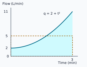
The endpoint mean is L/min, which would overestimate the delivered amount. The average rate of change of the flow is L/min²: it describes how rapidly the flow increases, not how much water arrives per minute.
Four graduated practice questions
1. Interval width matters
Find the average value of on , using dimensionless coordinates.
Hint
The interval width is 2, not 3. Integrate before dividing.
Explained solution
The value lies between 1 and 9. Dividing by the upper endpoint instead would give , which uses the wrong width. The equal-area rectangle has width 2 and height .
2. Compare all three quantities
For on , find the endpoint mean and average rate of change. Compare them with Question 1, then find where the function attains its integral average.
Hint
Endpoint mean adds function values; slope subtracts them. For the attainment point, solve inside the interval.
Explained solution
The endpoint mean is ; the average rate of change is ; the integral average is . These are different questions, even with dimensionless coordinates. The point is , approximately 2.08. The negative root is outside the interval. A secant slope of 4 does not mean that the average height is 4.
3. Weight unequal time intervals
A pump runs at 4 L/min for 2 minutes, then 10 L/min for 1 minute. Find the average flow over all 3 minutes. Must the pump ever run at that average?
Hint
Compute each amount separately. The two flow rates last different lengths of time.
Explained solution
The total is L, so the average is L/min. The unweighted mean 7 L/min is wrong because the durations differ. This piecewise-constant pump only runs at 4 or 10 L/min, so it need not attain 6 L/min. There is a jump: the continuity guarantee does not apply.
4. Signed velocity versus speed
An object has velocity m/s for seconds; t is numerical time in seconds. Find its average velocity and average speed.
Hint
Average velocity uses signed displacement; average speed uses total distance. Split the absolute-value integral at .
Explained solution
The displacement and average velocity are therefore zero. Distance is The object travels 4 m, so its average speed is 1 m/s. Zero average velocity does not mean no motion. The equal-signed-area height for velocity is zero, while the speed graph stays nonnegative.
Before moving on, say what you averaged, identify the interval width, and state the answer’s units. Return to the worked model.
For help choosing a method or setting up an area or volume, see Concordia MATH 205 tutoring. Ready to work without hints? Try the nine-question MATH 205 midterm mock. For McGill MATH 141, choose questions that match your current course outline.
Course topics and exam information
Concordia Fall 2026: scope and assessment arrangements
The Fall 2026 outline lists the common MATH 205 midterm for Sunday, November 1, 2026, 14:00–15:30 local time, covering weeks 1–6. Check your instructor’s announcements for the room and any changes.
Workshop: read an accumulation from a graph
A graph can define an integrand exactly, even when no single formula is supplied. Here you will calculate signed contributions, then use the same graph to describe the accumulated function. These original questions practise interpretation, not a prediction of an assessment. Allow about 20 minutes; try the checks before opening their hints.
One graph, two different functions
Let be continuous on , with straight segments joining the listed points in order. Define . Coordinates are dimensionless. The table and straight-segment instruction define every value, not just measured samples; the geometric integrals below are exact.
| 0 | 2 |
| 2 | 4 |
| 4 | 0 |
| 6 | −2 |
| 8 | 2 |
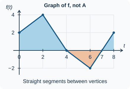
For a straight segment of width with endpoint heights , its signed integral is . Alternatively, split at a zero and use triangles. A negative integral is not a negative geometric area: it records a contribution below the axis. Reversing the bounds reverses the integral’s sign.
Worked example 1: accumulate, rather than count only positive area
Find and compare it with . First locate the extra zero: the segment from to reaches zero halfway, at .
From 0 to 2, the trapezoid contributes . From 2 to 4, the triangle contributes . From 4 to 6, subtract . The triangles on and contribute −1 and +1.
In contrast, . The two final triangles cancel in the signed integral, but both count positively for total geometric area. A useful running check is , , , , , . These are accumulated values, not heights of the displayed graph.
Read change from height; read concavity from slope
The fundamental theorem gives for , because is continuous. Thus positive graph heights mean that increases; negative heights mean it decreases. Where is differentiable, : rising graph segments make concave up, and falling segments make it concave down.
Worked example 2: extrema are not peaks of the displayed graph
Classify on the full domain. It increases on , decreases on , and increases on . The sign changes therefore give a local maximum at and a local minimum at . Comparing their values with both endpoints gives the absolute maximum and absolute minimum . The local minimum 7 is not the smallest value overall.
Concavity changes at 2 and 6: is concave up on and , and concave down on . Although has a corner at 4, it keeps decreasing there, so has no inflection at 4. Its second derivative is undefined there, but its first derivative exists. At 2, the peak of means a largest positive slope of , not a maximum of .
Four graduated checks
1. Stop between two vertices
Find , then .
Hint
Read the height at 1 from the straight segment. Subtract accumulated values to change the lower bound.
Explained solution
Linear interpolation gives . Thus , and . The height 3 and accumulated value answer different questions.
2. Reverse the interval
Find . Explain the sign.
Hint
First calculate from 2 to 6, keeping the negative triangle.
Explained solution
From 2 to 6 the net contribution is . Reversing gives . Equivalently, . The reversed orientation, not an entirely negative graph, explains this sign.
3. Separate height from slope
Find and . Is increasing or decreasing, and with which concavity?
Hint
One answer is the height of ; the other is its segment slope.
Explained solution
The height is , and the slope is . Hence and : is decreasing and concave down locally. The equal numbers are coincidental; they represent different measurements.
4. Move the endpoint backward
Let for . Find and , and explain why the derivative is positive.
Hint
The endpoint is 6 when , and its rate is −2. Shrinking an interval can remove a negative contribution.
Explained solution
We have . The chain rule gives , so . Near this endpoint, moving backward removes negative signed area, increasing the accumulation. The corner of at 6 does not prevent this derivative: continuity of is enough.
Final check: say whether each step uses a height, a slope, or a signed area. That distinction is more reliable than treating every feature of as the same feature of .
Further reading: OpenStax: the fundamental theorem of calculus explains the continuity condition and the derivative of an accumulation. The questions and graph in this workshop are original.
Useful for
Concordia MATH 205: integration methods, areas and volumes. Also useful for overlapping topics in McGill MATH 141.
Work on the step you’re missing.
Tell us the subject and your preferred time. Nablio confirms the details by text or email.
Request a lesson