Surface flux with oriented area vectors and closing surfaces

Flux and orientation

For an oriented surface $S$, write

Here $\mathbf n$ is a unit normal, and $dS$ is a positive surface-area element. The dot product selects the component of the field perpendicular to the surface. A positive contribution points with the chosen normal; a negative contribution points against it. A tangent field contributes zero at that point.

Choosing the opposite normal reverses the sign of the flux. It does not change the surface area. A zero integral can mean that positive and negative contributions cancel; it does not establish that the field vanishes.

An open surface needs a stated orientation, such as upward or toward the positive x direction. “Outward” is meaningful when a reference solid has been specified. For a closed boundary, outward means away from the enclosed solid, including into any cavity.

A disk includes its circular edge but is still an open surface in this calculus terminology: it has a boundary curve and does not enclose a solid by itself. Here “closed surface” means a complete enclosing boundary, not merely a closed set of points.

Build the area vector from two parameters

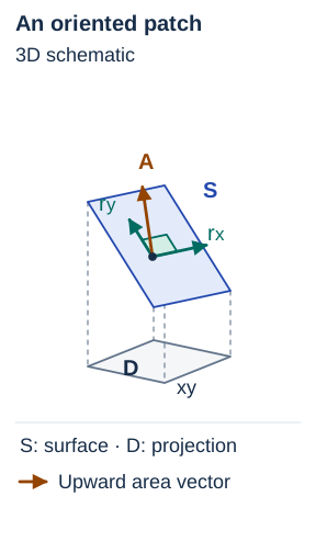
Let $\mathbf r(u,v)$ describe $S$ once over a parameter region $D$, apart from shared edges or coordinate seams. Its partial derivatives $\mathbf r_u$ and $\mathbf r_v$ are tangent to the surface. Their cross product is normal to it:

For a regular patch, $\mathbf A\ne\mathbf0$. The cross-product magnitude converts parameter area into surface area. It generally varies across the patch.

If $\mathbf A$ points in the required direction, then

so

For each connected regular patch with a continuous chosen orientation, check the sign at an easy point. The relative sign cannot change on that patch without losing regularity or continuity. Check disconnected patches separately. For an upward orientation, the z component of the area vector must be positive. For an outward sphere, its dot product with a radial outward vector must be positive. If the cross product points the wrong way, negate it or reverse the cross-product order, but do not do both.

There are two consistent ways to calculate: use a unit normal together with $dS$, or use the unnormalized cross product with $du\,dv$. Normalizing the cross product while retaining only $du\,dv$ loses its area scale. Multiplying the unnormalized cross product by a second $\|\mathbf A\|$ counts that scale twice.

A single chart need not work everywhere. Spherical coordinates, for example, degenerate at a pole. One can use regular patches and a limit; the pole and coordinate seam do not change the ordinary surface integrals used here. Do not use a parameterization that covers a positive-area part twice.

Use the graph formula carefully

For $z=g(x,y)$ over a region $D$ in the xy plane, choose

Then

Its last component is positive, so this is the upward area-vector density. The downward one is $(g_x,g_y,-1)$.

For $\mathbf F=(P,Q,R)$, the upward flux is

Evaluate every field component on the surface before simplifying. The corresponding scalar area is $\iint_D\sqrt{1+g_x^2+g_y^2}\,dx\,dy$; it is a different integral.

Worked patch

Take $z=x+y$, $0\le x\le1$, $0\le y\le1$, upward orientation, and $\mathbf F=(1,0,2)$. The area-vector density is $(-1,-1,1)$, so

Check with the other convention: the unit normal is $(-1,-1,1)/\sqrt3$ and the patch area is $\sqrt3$. Their factors cancel, giving $(1/\sqrt3)\sqrt3=1$. The downward flux is $-1$.

If you change the projection coordinates to polar coordinates, the planar area element also changes: $dx\,dy=\rho\,d\rho\,d\theta$. This factor belongs to the change of variables in the projection plane. It is not an extra surface-area factor to attach after a full polar cross product has already been computed.

Try question 1 on a tilted patch, then question 2 on a curved graph.

Check the divergence theorem conditions

For the usual introductory form, let $E$ be a bounded solid with a closed, piecewise-smooth boundary $\partial E$. Assume $\mathbf F$ has continuous first partial derivatives on an open set containing the whole solid and its boundary. With outward normals,

Check these three things before using the equality:

1. The surface on the left contains the entire boundary of the solid on the right.
2. Every boundary piece uses the outward normal for that same solid.
3. The field satisfies the differentiability condition throughout a neighbourhood of the solid, including its interior.

A polynomial field meets the third condition everywhere. A field with a denominator that vanishes inside the solid needs a separate domain check, even when it is smooth on the outer surface. Computing divergence only where a formula is defined does not repair a missing hypothesis.

If you need a closed-boundary starting example, return to the MAST 219 box calculation. It explicitly adds all six faces. Question 6 shows why a singularity inside a sphere matters.

Close an open surface and subtract the signed contribution

Suppose an open surface $S$ and an added surface $B$ together form $\partial E$. They may meet along an edge, but their interiors must not overlap. Orient both outward from $E$. Then

The quantity subtracted is the signed flux through the added surface. Subtracting a negative cap contribution increases the result. If several pieces are needed to close the surface, subtract their sum. If the requested orientation of $S$ is inward, first obtain its outward flux and then reverse the sign.

Worked hemisphere with a nonzero closing disk

Let $S$ be the curved upper unit hemisphere

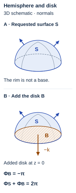
oriented away from the origin. The field is $\mathbf F=(x,y,z+1)$. The equatorial circle is the edge of $S$; the disk it bounds is not included in the requested flux.

Add the disk $B:\ z=0,\ x^2+y^2\le1$. Together they bound the upper half-ball $E$. The field is polynomial, the boundary is piecewise smooth, and $\nabla\cdot\mathbf F=3$. Therefore the total outward flux is

On the disk, the outward normal points down because the solid lies above it. Thus $\mathbf n_B=(0,0,-1)$. At $z=0$, the field is $(x,y,1)$, giving $\mathbf F\cdot\mathbf n_B=-1$. Consequently,

Reporting $2\pi$ would give the flux through the hemisphere and disk together. Reporting $\pi$ would subtract the disk's unsigned magnitude instead of its signed flux.

Verify the hemisphere directly

Use colatitude $\varphi$, measured down from the positive z axis, and azimuth $\theta$:

The outward unit normal on the unit sphere is $\mathbf r$. In this parameter order,

Its radial dot product is positive for $0<\varphi\le\pi/2$, and $dS=\sin\varphi\,d\varphi\,d\theta$. Since

we obtain

The direct calculation and the closing-disk method agree. Both account for the hemisphere only and use the same orientation. For a changed boundary above the equator, try question 4.

Recognize which integral the question asks for

A scalar surface integral such as $\iint_S 1\,dS$ measures area and does not use an orientation. The flux $\iint_S\mathbf F\cdot\mathbf n\,dS$ does use one. A line integral $\int_C\mathbf F\cdot d\mathbf r$ follows an oriented curve and measures a different quantity.

The divergence theorem relates flux of $\mathbf F$ across a closed boundary to divergence inside a solid. Stokes' theorem relates circulation along a boundary curve to flux of $\nabla\times\mathbf F$ through a compatible oriented surface. An open surface can be used in Stokes, but that does not turn an arbitrary flux of $\mathbf F$ into a circulation calculation.

If the original question follows a curve, use the existing line-integral setup lesson. For the cylindrical side in question 3, a direct parameterization is short and also makes a two-cap check possible.

Repair the first unsupported step

• Wrong sign: write the requested normal direction and test your cross product at one point.
• Wrong magnitude: identify whether your normal is unit length and where the area factor appears.
• Wrong domain: distinguish the parameter region, the projection region, the surface and the enclosed solid.
• Missing cap: list every boundary piece and keep its signed contribution until the final subtraction.
• Invalid theorem: check the field's domain on the whole solid before integrating its divergence.

Try the six progressive flux questions. Bring a sketch and the first step you cannot justify to a tutor. Work through the correction, then set up a changed problem without the solution.

Course connections and references

This lesson supports selected surface-integral and Gauss/divergence topics in Concordia MAST 219 and Concordia ENGR 233. Choose it when your current chapter covers surfaces and flux. It is independent practice and makes no claim about a particular assessment or its timing.

Curriculum scope was checked on 11 October 2026 against Concordia's mathematics calendar and engineering calendar. The OpenStax surface-integral section and divergence-theorem section provide further reference. The worked examples here were written for Nablio.