A Wave in Space and Time

Reading a wave in space and in time

A wave graph can show the shape of a whole string at one instant, or the motion of one small part of the string as time passes. Begin with the horizontal axis: it tells you which question the graph answers.

This example uses an ideal sinusoidal transverse wave travelling to the right on a uniform string. “Transverse” means that each small part of the string moves up and down, perpendicular to the direction of propagation. We neglect damping and reflections, and treat the profile as translating without changing shape. In this ideal model, each particle keeps its horizontal coordinate. A particle means a small tagged part of the string, not a crest.

Two graphs of the same wave

Let $x$ denote horizontal position along the string, measured to the right in metres. Let $t$ denote time in seconds. The displacement $y$ is the signed vertical displacement from equilibrium: positive above equilibrium and negative below it. We write $y(x,t)$ because the displacement depends on both position and time. The graphs show $y$ in centimetres.

Tag the particle at $x=0$ and call it $P$. Choose $t=0$ to be an instant when $P$ is at the top of its motion. The string continues on either side of the plotted segment; $x=0$ is a coordinate choice, not a fixed end.

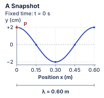
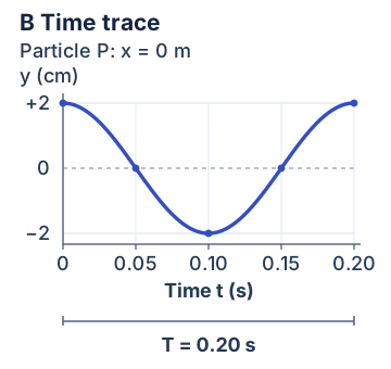
The two curves have the same shape on the page because the horizontal scales were chosen to show one complete cycle. Their axes carry different units. On A, moving right along the graph means looking farther along the string. On B, it means waiting longer while watching $P$.

Read amplitude and wavelength from the snapshot

The amplitude $A$ is the largest distance a particle moves away from equilibrium. The crest is $2.0\,\mathrm{cm}$ above equilibrium and the trough is $2.0\,\mathrm{cm}$ below it, so

$$A=2.0\,\mathrm{cm}=0.020\,\mathrm m.$$

The full vertical distance from a crest to a trough is $2A=4.0\,\mathrm{cm}$. It is twice the amplitude.

The wavelength $\lambda$, pronounced “lambda,” is the horizontal length of one complete repetition of the profile. On Figure A, the crest at $x=0$ and the next crest at $x=0.60\,\mathrm m$ give

$$\lambda=0.60\,\mathrm m.$$

A crest and the adjacent trough are only half a wavelength apart: $0.30\,\mathrm m$. To measure a full wavelength, choose two successive points at the same stage of the pattern, such as two crests.

A single snapshot gives spatial information. By itself, it does not tell us how quickly the wave travels, which direction it travels, or how long one particle takes to complete a cycle. Rightward travel is part of this example's stated model, not something deduced from Figure A alone.

Read period and frequency from the time trace

The period $T$ is the time for one complete oscillation of a particle. In Figure B, $P$ is at its upper turning point at $t=0$ and again at $t=0.20\,\mathrm s$. Therefore

$$T=0.20\,\mathrm s.$$

Between those two instants, the particle passes through equilibrium moving downward at $0.05\,\mathrm s$, reaches its lower turning point at $0.10\,\mathrm s$, and passes through equilibrium moving upward at $0.15\,\mathrm s$.

The frequency $f$ is the number of complete oscillations per second. One cycle takes $T$ seconds, so

$$\begin{aligned} f&=\frac{1}{T}\\ &=\frac{1}{0.20\,\mathrm s}\\ &=5.0\,\mathrm{Hz}. \end{aligned}$$

One hertz, written $\mathrm{Hz}$, means one cycle per second. Frequency and period describe the same repetition in reciprocal ways: five cycles fit into one second, so one cycle takes one fifth of a second.

The crossings at $0.05\,\mathrm s$ and $0.15\,\mathrm s$ have the same displacement, but opposite directions of motion. Their separation is $T/2$, not a full period. A complete cycle returns the particle to the same displacement and the same stage of its motion.

Connect the two graphs with propagation speed

Let $v$ denote the positive speed at which this wave profile travels. Track one crest as it moves right. In one period, the profile has advanced by one wavelength: the next identical crest then reaches any fixed observation point. Distance divided by elapsed time gives

$$\begin{aligned} v&=\frac{\lambda}{T}\\ &=\frac{0.60\,\mathrm m}{0.20\,\mathrm s}\\ &=3.0\,\mathrm{m/s}. \end{aligned}$$

Since $f=1/T$, this is also $v=f\lambda$. The units agree: $\mathrm{s^{-1}}$ multiplied by $\mathrm m$ gives $\mathrm{m/s}$.

Here, both graphs are needed: the snapshot provides $\lambda$, and the time trace provides $T$. A time trace alone does not give the distance between neighbouring crests.

Follow a crest and follow a particle

At $t=0$, particle $P$ happens to sit at a crest. The crest travels right at $3.0\,\mathrm{m/s}$. Particle $P$ stays at $x=0$ and moves vertically.

Let $\Delta x$ mean the change in the crest’s horizontal position, and $\Delta t$ the elapsed time. After a quarter-period, $0.05\,\mathrm s$, the crest has moved a horizontal distance

$$\begin{aligned} \Delta x&=v\,\Delta t\\ &=(3.0\,\mathrm{m/s})(0.05\,\mathrm s)\\ &=0.15\,\mathrm m. \end{aligned}$$

The particle at $x=0.15\,\mathrm m$ now occupies that crest. Meanwhile, Figure B tells us that $P$ has moved down from $+2.0\,\mathrm{cm}$ to equilibrium. Following a crest takes us from one particle to another; following $P$ keeps us at one horizontal coordinate.

Why is the particle momentarily stationary at a crest? Look at its time trace. At a smooth upper turning point, the trace has a horizontal tangent: the particle changes from moving upward to moving downward. Its instantaneous vertical velocity is zero at that instant. It does not remain there for a finite time.

The moving crest is a location of maximum displacement in the profile. It can move steadily to the right while the particular particle occupying that location has zero instantaneous velocity. There is no contradiction: the two velocities describe different motions.

A snapshot's slope describes how displacement changes with position. A time trace's slope describes how displacement changes with time. Use the second graph when reading the particle's instantaneous vertical velocity. A flat point on an arbitrary snapshot alone is not enough to establish a particle's velocity without information about how the profile evolves.

Optional: Build a wave equation from the graphs

This section uses radians and the cosine function. You can use the two graphs without it.

Cosine begins at its maximum: $\cos 0=1$. It completes one cycle when its argument increases by $2\pi$ radians. In the snapshot, $x/\lambda$ counts how many wavelengths we have moved along the string. Multiplying that number by $2\pi$ turns it into the cosine argument. Multiplying by $A$ sets the vertical scale:

$$y(x,0)=A\cos\!\left(2\pi\frac{x}{\lambda}\right).$$

For example, $x=\lambda/2$ gives $\cos\pi=-1$, so the midpoint of the plotted cycle is a trough with displacement $-A$.

After time $t$, the whole profile has shifted right by the distance $vt$. The displacement now at position $x$ is the displacement that the original profile had at $x-vt$. Replace $x$ in the snapshot by $x-vt$:

$$y(x,t)=A\cos\!\left(2\pi\frac{x-vt}{\lambda}\right).$$

Because $v=\lambda/T$, the same equation can be written as

$$\begin{aligned} &y(x,t)\\ &=A\cos\!\left[2\pi\left(\frac{x}{\lambda}-\frac{t}{T}\right)\right]. \end{aligned}$$

Both $x/\lambda$ and $t/T$ are dimensionless. The minus sign describes rightward translation: as time increases, $x$ must also increase to keep a particular crest at the same value of the cosine argument. This sign is tied to our choice of positive $x$ to the right.

At $x=0$, the expression becomes $A\cos(-2\pi t/T)$. Cosine is even, meaning $\cos(-z)=\cos z$ for any angle $z$. Thus the motion of $P$ is

$$y(0,t)=A\cos\!\left(2\pi\frac{t}{T}\right),$$

which reproduces Figure B. A leftward translation of this same starting profile would give a plus sign inside the wave equation and the same time trace at $x=0$, because cosine is even. Therefore, this particular pair of graphs does not determine the direction; our rightward model does.

If you have studied derivatives

Let $u_P(t)$ denote the signed vertical velocity of particle $P$, positive upward. Differentiating its displacement with respect to time gives

$$\begin{aligned} u_P(t)&=\frac{d}{dt}\,y(0,t)\\ &=-\frac{2\pi A}{T}\sin\!\left(2\pi\frac{t}{T}\right). \end{aligned}$$

At the crest, $t=0$, the sine factor is zero, so $u_P(0)=0$. At $t=T/4$, the particle crosses equilibrium downward and its vertical velocity is

$$\begin{aligned} u_P(T/4)&=-\frac{2\pi(0.020\,\mathrm m)}{0.20\,\mathrm s}\\ &=-0.20\pi\,\mathrm{m/s}\\ &\approx-0.63\,\mathrm{m/s}. \end{aligned}$$

The negative sign means downward. The particle's maximum speed is $2\pi A/T$, about $0.63\,\mathrm{m/s}$; the wave's propagation speed is $3.0\,\mathrm{m/s}$. One measures vertical oscillation; the other measures horizontal travel of the profile.

Three self-checks

1 Read the axes before calculating

In Figure A, the vertical distance from crest to trough is $4.0\,\mathrm{cm}$, and the horizontal distance from a crest to the adjacent trough is $0.30\,\mathrm m$. Find the amplitude and wavelength. Can Figure A alone give the period?

Show the explained solution

The crest-to-trough vertical span is $2A$, so $A=2.0\,\mathrm{cm}$. The crest-to-adjacent-trough horizontal span is $\lambda/2$, so $\lambda=0.60\,\mathrm m$. No period can be read from this snapshot alone because its horizontal axis gives position, not elapsed time. Figure B supplies $T=0.20\,\mathrm s$.

2 Track two different motions

Starting at $t=0$, wait $0.10\,\mathrm s$. Where is the crest that started at $x=0$? What are the horizontal coordinate and vertical displacement of particle $P$? Is $P$ moving vertically at that instant?

Show the explained solution

The crest moves right by

$$\Delta x=(3.0\,\mathrm{m/s})(0.10\,\mathrm s)=0.30\,\mathrm m.$$

Its new position is $x=0.30\,\mathrm m$. Particle $P$ still has horizontal coordinate $x=0$. Half a period has passed, so Figure B gives $y(0,0.10\,\mathrm s)=-2.0\,\mathrm{cm}$: $P$ is at its lower turning point. Its instantaneous vertical velocity is zero there. The crest has travelled horizontally while $P$ has moved downward by $4.0\,\mathrm{cm}$.

3 Predict what changes in the same medium

For a new wave on the same ideal nondispersive string, keep propagation speed at $3.0\,\mathrm{m/s}$ and amplitude at $2.0\,\mathrm{cm}$, but double the frequency. “Nondispersive” means that, under these unchanged conditions, propagation speed does not depend on frequency. Find the new period and wavelength. How should the two graphs change?

Show the explained solution

The new frequency is $10\,\mathrm{Hz}$. Let $T_{\mathrm{new}}$ and $\lambda_{\mathrm{new}}$ denote the new period and wavelength. Then

$$\begin{aligned} T_{\mathrm{new}}&=\frac{1}{10\,\mathrm{Hz}}\\ &=0.10\,\mathrm s,\\[4pt] \lambda_{\mathrm{new}}&=\frac{3.0\,\mathrm{m/s}}{10\,\mathrm{Hz}}\\ &=0.30\,\mathrm m. \end{aligned}$$

On the same horizontal scales, Figure A would show crests half as far apart, and Figure B would show maxima half as far apart in time. Both graphs would keep the same amplitude. The profile's speed is unchanged; a higher frequency alone has not made it travel faster.

If using the derivative extension, the particle's maximum speed doubles to $0.40\pi\,\mathrm{m/s}$, about $1.26\,\mathrm{m/s}$, because $2\pi A/T_{\mathrm{new}}$ describes the same vertical motion completed in half the time.

A short method to reuse

1. Name both axes and check their units.
2. State what stays fixed: time for a snapshot, position for a time trace.
3. Read amplitude vertically; read wavelength or period horizontally.
4. Identify what moves before calculating a velocity: a particle or a feature of the profile.

This is an original practice example. Use the assumptions stated in your own problem when extending it to sound, standing waves, or optical phenomena.