Electric Field vs Electric Potential: Signs, Units and Worked Examples

Nablio · 35 minPublished October 3, 2026

Stuck on a step? Text us Email us Request a lesson

Electric field tells you the electric force per unit charge at a location. Electric potential tells you the electric potential energy per unit charge, relative to a chosen zero. The distinction becomes useful as soon as several charges contribute: field contributions add as vectors; potential contributions add as signed numbers.

Before you start: be comfortable with signed numbers, scientific notation, vectors along a line and the idea of work. The main examples use algebra. Optional calculus connections use derivatives to explain $\vec E=-\nabla V$ and a line integral to express a potential difference.

By the end: you should be able to choose among field, potential, force and energy; explain their signs and units; combine two source charges; and read a field direction from a potential graph. The original examples support the field-and-potential topics listed for Concordia PHYS 205 and McGill PHYS 102. This is a focused lesson, not a complete course or an assessment guide. Use your current section outline to choose your next problems.

1. Choose the quantity before the formula

Use capital $Q_i$ for a source charge: one of the charges creating the field. Use lower-case $q$ for a test charge placed at the point being studied. A test charge can be positive or negative. We assume the sources remain fixed and that the test charge does not appreciably change their arrangement. The field and potential below are due to the sources, excluding the test charge’s own field.

Electric field $\vec E$ : a vector describing electric force per unit positive test charge. Its SI unit is the newton per coulomb, N/C. Its direction is the direction of the electric force on a positive test charge.
Electric potential $V$ : a scalar describing potential energy per unit charge, with a stated reference. Its SI unit is the volt: $1\,\mathrm{V}=1\,\mathrm{J/C}$ . A scalar can be negative; it has no spatial direction.
Electric force $\vec F_{\mathrm e}$ : a vector acting on the particular charge $q$ . Its unit is the newton, N.
Electric potential energy $U$ : an energy associated with the interaction between $q$ and the fixed sources. Its unit is the joule, J. It is not simply a property of an isolated particle.

\vec F_{\mathrm e}=q\vec E

U=qV

The energy equation uses consistent zero references for $U$ and $V$ ; potential differences give the reference-independent relation $\Delta U=q\Delta V$ . Doubling $q$ doubles the force and interaction energy. It does not double the source field or potential. Changing the sign of $q$ reverses the electric force and the sign of $U$ for the same chosen reference.

For $q<0$ , force points opposite the field. A field arrow does not show a particle’s velocity: an already moving particle can have a velocity in a different direction from its force. See OpenStax’s electric-field definition for the source/test-charge distinction.

2. Calculate field and potential from one source

For an isolated, fixed point charge $Q$ in vacuum, choose $V\to0$ as the distance tends to infinity. At distance $r>0$ ,

V=\frac{kQ}{r}

\vec E=\frac{kQ}{r^2}\,\hat r

Here $\hat r$ is a unit vector pointing from the source to the observation point. The distance $r$ is always positive; the sign belongs to $Q$ . We use the rounded value $k=9.0\times10^9\,\mathrm{N\,m^2/C^2}$ throughout the numerical examples. These point-charge formulas do not apply at the source itself, $r=0$ .

If $Q>0$ , potential is positive under this reference and field points away from the source. If $Q<0$ , potential is negative and field points toward the source. The field magnitude is $k|Q|/r^2$ , which is never negative. A component such as $E_x$ can be negative because it indicates direction along a chosen axis.

Worked example: a negative test charge near a positive source

Place $Q=+4.0\,\mathrm{nC}$ at the origin. Point $P$ is 0.30 m to its right. Take right as positive and remember $1\,\mathrm{nC}=10^{-9}\,\mathrm C$ . First calculate the source quantities at $P$ :

In SI units, the common product is $kQ=36\,\mathrm{N\,m^2/C}$ . This keeps the arithmetic in short steps:

\begin{aligned}V(P)&=\frac{36}{0.30}\,\mathrm V\\&=+1.2\times10^2\,\mathrm V.\end{aligned}

\begin{aligned}E_x(P)&=\frac{36}{(0.30)^2}\,\mathrm{N/C}\\&=+4.0\times10^2\,\mathrm{N/C}.\end{aligned}

Now place $q=-2.0\,\mathrm{nC}$ at $P$ . This second step answers questions about that test charge:

\begin{aligned}F_{\mathrm e,x}&=qE_x\\&=(-2.0\times10^{-9})(400)\\&=-8.0\times10^{-7}\,\mathrm N,\end{aligned}

\begin{aligned}U&=qV\\&=(-2.0\times10^{-9})(120)\\&=-2.4\times10^{-7}\,\mathrm J.\end{aligned}

The field is rightward, the force on the negative test charge is leftward, and the interaction energy is negative relative to infinite separation. There is no contradiction: the four answers describe different quantities.

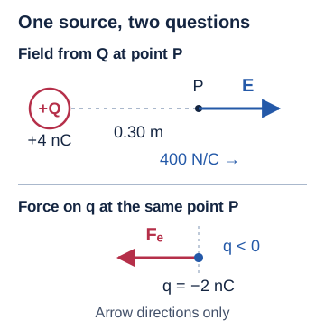
A positive source is left of point P. Its electric field at P points right. In a separate row, the electric force on a negative test charge at the same point P points left. The source field remains unchanged. — Figure 1. Field and force directions at the same location. The two rows separate the source field from the response of the negative test charge. Arrow lengths do not compare quantities with different units.

Distance check: doubling $r$ halves $V$ and quarters the field magnitude. The factors differ because potential varies as $1/r$ and field magnitude as $1/r^2$ .

3. Explain two different kinds of cancellation

With several fixed point sources, calculate each contribution using its own distance $r_i>0$ . For a finite set of these sources, keep the common reference $V\to0$ at infinity:

V=\sum_i\frac{kQ_i}{r_i}

\vec E=\sum_i\frac{kQ_i}{r_i^2}\,\hat r_i

Potential adds algebraically, including charge signs. Field adds vectorially, including directions. For charges on the $x$ -axis, mark each field arrow before assigning a signed $x$ -component. The sign of a source alone does not determine the sign of its field component: the observation point’s position also matters. This way of adding contributions is called superposition. It is explained in OpenStax’s point-charge potential treatment.

Put equal-magnitude sources at $x=-a$ and $x=+a$ , where $a>0$ , and examine their midpoint $M$ . Let $Q>0$ denote the common charge magnitude.

Case A: two positive sources, $+Q$ and $+Q$

The left source produces a rightward field at $M$ ; the right source produces an equally strong leftward field. They cancel. Their potentials have the same positive sign and add:

E_x(M)=\frac{kQ}{a^2}-\frac{kQ}{a^2}=0

V(M)=\frac{kQ}{a}+\frac{kQ}{a}=\frac{2kQ}{a}

For $Q=2.0\,\mathrm{nC}$ and $a=0.20\,\mathrm m$ , each field contribution has magnitude 450 N/C and each potential contribution is +90 V. Thus $\vec E(M)=\vec0$ , while $V(M)=+180\,\mathrm V$ .

Case B: a positive left source and a negative right source

The left source’s field points away from $+Q$ , to the right. The right source’s field points toward $-Q$ , also to the right. Their fields add; their equal and opposite potentials cancel:

E_x(M)=\frac{kQ}{a^2}+\frac{kQ}{a^2}=\frac{2kQ}{a^2}

V(M)=\frac{kQ}{a}-\frac{kQ}{a}=0

With the same numbers, $E_x(M)=+900\,\mathrm{N/C}$ , while $V(M)=0$ . A nonzero test charge at this zero-potential point still experiences an electric force.

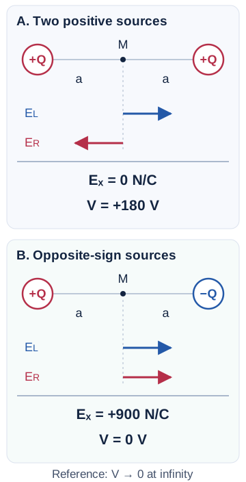
Two vertically stacked midpoint diagrams use sources at equal distances from M. With two positive sources, equal field arrows at M point oppositely, giving zero net field and positive potential. With positive left and negative right sources, both field arrows at M point right, giving positive net field and zero potential. Potentials use zero at infinity. — Figure 2. The sources lie 0.20 m from the midpoint. Field contributions at M are shown in separate rows for clarity; every contribution has the same magnitude, 450 N/C. In both panels the potential reference is zero at infinity.

What the zeros mean: zero field at one point says the electric forces cancel there. It does not say the potential is zero, or that the field vanishes nearby. Zero potential says the scalar sum equals the chosen reference. It does not say the potential is locally flat.

In Case A, a test charge has zero electric force exactly at $M$ . This alone does not establish stable equilibrium: stability requires considering small displacements in all allowed directions, as well as any other forces or constraints.

4. Read field from the slope of potential

The height of a potential graph gives $V$ ; its spatial slope gives a component of $\vec E$ . In a region with a uniform field along the $x$ -direction,

E_x=-\frac{\Delta V}{\Delta x}

Here $\Delta x=x_B-x_A$ is a signed displacement and $\Delta V=V_B-V_A$ . A potential that decreases as $x$ increases gives $E_x>0$ . The field points in the direction of decreasing potential. The field unit can therefore also be written V/m; $1\,\mathrm{V/m}=1\,\mathrm{N/C}$ .

Read a straight-line potential graph

In the region shown, potential is 120 V at $x=0$ , 80 V at $x=0.20\,\mathrm m$ , and 40 V at $x=0.40\,\mathrm m$ . The line is straight, so the field component is constant throughout the interior of that region:

\begin{aligned}E_x&=-\frac{40-120}{0.40-0}\\&=+200\,\mathrm{V/m}.\end{aligned}

The graph slopes downward to the right, so the field points right. A negative test charge feels a force to the left. This graph gives the $x$ -component; to infer the complete field, we assume potential has no dependence on the other coordinates in this example.

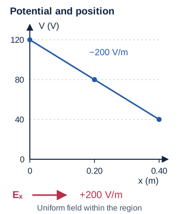
A potential versus position graph is a straight line through 0 metres and 120 volts, 0.20 metres and 80 volts, and 0.40 metres and 40 volts. Its slope is minus 200 volts per metre, so the electric field points right with x component plus 200 volts per metre. — Figure 3. A negative slope produces a positive field component. The graph describes a finite region; it does not impose a zero-at-infinity reference for an everywhere-uniform field.

Changing the zero leaves the field unchanged

Subtract 80 V from every potential value. The graph now passes through +40 V, 0 V and −40 V at the same three positions. Its slope and every potential difference stay the same. At $x=0.20\,\mathrm m$ , the new potential is zero but the field is still rightward at 200 N/C.

In general, adding a constant to $V$ changes the chosen reference, not the field. For point charges, $V=kQ/r$ specifically uses zero at infinity; another reference adds a constant.

Optional calculus: from a slope to a gradient

If the field varies along a straight displacement in the $x$ -direction, the quotient $-\Delta V/\Delta x$ gives the average x-component over that displacement, not necessarily the field at a particular point. At a smooth point, use the local slope:

E_x=-\frac{dV}{dx}

When $V$ depends on several coordinates, use a partial derivative for each component. The vector that collects those derivatives is the gradient:

\vec E=-\nabla V

E_x=-\frac{\partial V}{\partial x},\quad E_y=-\frac{\partial V}{\partial y}

E_z=-\frac{\partial V}{\partial z}

For a point charge, the radial derivative of $kQ/r$ is $-kQ/r^2$ ; applying the extra minus sign recovers the radial field component $kQ/r^2$ . These relations apply here to electrostatic fields. A general electric field associated with a changing magnetic field cannot be described by a scalar potential alone. See OpenStax’s field-from-potential discussion.

5. Convert potential difference into work and energy

For a test charge $q$ moving from $A$ to $B$ among fixed sources, begin with the potential difference. Keep the order “final minus initial”:

\Delta V=V_B-V_A

\Delta U=q\Delta V

W_{\mathrm e}=-\Delta U

Here $W_{\mathrm e}$ is work done by the electric force. If that is the only force doing work, the work–energy theorem gives $\Delta K=W_{\mathrm e}$ . If you move the charge slowly so its kinetic energy does not change, and no other non-electric force does work apart from your applied force, your external work is instead $W_{\mathrm{ext}}=\Delta U$ .

Worked example: moving through an 80 V drop

Use $V_A=120\,\mathrm V$ , $V_B=40\,\mathrm V$ , and $q=+3.0\,\mathrm{nC}$ . The potential difference is $-80\,\mathrm V$ , so

\begin{aligned}\Delta U&=q\Delta V\\&=(3.0\times10^{-9})(-80)\\&=-2.4\times10^{-7}\,\mathrm J,\end{aligned}

W_{\mathrm e}=+2.4\times10^{-7}\,\mathrm J.

The interaction loses potential energy and the electric force does positive work. If electric force alone does work, kinetic energy increases by the same amount. Slow controlled transport would require external work of $-2.4\times10^{-7}\,\mathrm J$ .

Now change only the test charge to $-3.0\,\mathrm{nC}$ . The potential difference remains −80 V, but $\Delta U=+2.4\times10^{-7}\,\mathrm J$ and electric work is negative. A negative charge does not spontaneously accelerate along the field from rest; its electric force is opposite the field. To reach B under electric force alone it would need enough initial kinetic energy.

Optional integral connection. If you know line integrals, an electrostatic potential difference can also be written as the negative line integral of the electric field along a path:

V_B-V_A=-\int_A^B\vec E\cdot d\vec\ell

The dot product selects the field component along each small displacement. In electrostatics, the result is independent of the path between the same endpoints. The constant-field formula in Section 4 is the straight-line special case. The OpenStax treatment of potential difference connects these energy and work definitions.

6. Solve a two-source problem away from the midpoint

Put $Q_L=+3.0\,\mathrm{nC}$ at $x=0$ , and $Q_R=-1.0\,\mathrm{nC}$ at $x=0.40\,\mathrm m$ . Find field and potential at $P$ , where $x=0.10\,\mathrm m$ . Keep zero potential at infinity and right as the positive direction.

Step 1: use distances from P to each source

The left distance is 0.10 m and the right distance is 0.30 m. The 0.40 m source separation is neither of these distances. Both field contributions point right: away from the left positive source and toward the right negative source.

Step 2: add signed potential contributions

\begin{aligned}V_L&=\frac{27}{0.10}\,\mathrm V\\&=+270\,\mathrm V,\end{aligned}

\begin{aligned}V_R&=\frac{-9}{0.30}\,\mathrm V\\&=-30\,\mathrm V.\end{aligned}

V(P)=270-30=+240\,\mathrm V

Step 3: add directed field components

The source charge signs are already accounted for by the directions. Use positive magnitudes for both rightward components:

\begin{aligned}E_{L,x}&=\frac{27}{(0.10)^2}\,\mathrm{N/C}\\&=+2700\,\mathrm{N/C},\end{aligned}

\begin{aligned}E_{R,x}&=\frac{9}{(0.30)^2}\,\mathrm{N/C}\\&=+100\,\mathrm{N/C}.\end{aligned}

E_x(P)=+2800\,\mathrm{N/C}

Subtracting 100 N/C because $Q_R$ is negative would count the source sign incorrectly. Its field points toward that source, which here means right.

Step 4: answer for a specific test charge only if needed

For $q=+2.0\,\mathrm{nC}$ ,

F_{\mathrm e,x}=+5.6\times10^{-6}\,\mathrm N

U=+4.8\times10^{-7}\,\mathrm J

These results describe the test charge’s interaction with the fixed sources. They do not include the mutual potential energy of the two sources, which is constant while the sources stay fixed.

7. Try five questions with hints and explanations

Use the same rounded $k$ . Unless a question changes it, keep the point-charge reference zero at infinity. Sketch the source positions, label every distance, and predict signs before calculating.

Question 1: change the test charge

At a point, $E_x=+600\,\mathrm{N/C}$ and $V=-90\,\mathrm V$ . Place $q=-2.0\,\mathrm{nC}$ there. Find electric force and interaction energy. What changes if you replace q with $+2.0\,\mathrm{nC}$ ?

Show a hint

Keep the source quantities fixed. Multiply the signed test charge by each one separately.

Show answer and reasoning

Initially, $F_{\mathrm e,x}=-1.2\times10^{-6}\,\mathrm N$ , so force is leftward, while $U=+1.8\times10^{-7}\,\mathrm J$ . With positive q, force becomes rightward at the same magnitude and U becomes negative with the same magnitude. The source field and potential remain +600 N/C and −90 V.

Question 2: change the source and distance

A source $Q=-2.0\,\mathrm{nC}$ is at the origin. Find potential and field at a point 0.30 m to its right. Then move the observation point to 0.60 m. Which quantity falls more quickly in magnitude?

Show a hint

The negative source pulls the field direction toward the origin at both points. Compare the factors $1/r$ and $1/r^2$ .

Show answer and reasoning

At 0.30 m, $V=-60\,\mathrm V$ and $E_x=-200\,\mathrm{N/C}$ . At 0.60 m, $V=-30\,\mathrm V$ and $E_x=-50\,\mathrm{N/C}$ . Potential magnitude halves and field magnitude quarters. Potential becomes less negative as you move right, so its positive slope is consistent with a leftward field.

Question 3: find zero field between unequal positive sources

Put $+2.0\,\mathrm{nC}$ at $x=0$ and $+8.0\,\mathrm{nC}$ at $x=0.60\,\mathrm m$ . Find the point between them where the field is zero. Is its potential also zero?

Show a hint

Between the sources the fields oppose. Set their magnitudes equal using distances x and $0.60-x$ , both positive.

Show answer and reasoning

For $0<x<0.60$ , cancellation requires

\frac{2.0}{x^2}=\frac{8.0}{(0.60-x)^2}.

Taking the positive square root of the distance ratio gives $0.60-x=2x$ . Thus $x=0.20\,\mathrm m$ , nearer the smaller source. Each field magnitude is 450 N/C. The potentials add:

V=90+180=+270\,\mathrm V.

Outside the interval, both fields point in the same direction, so there is no other finite zero on this axis. Zero field does not imply zero potential or stable equilibrium.

Question 4: find zero potential between opposite sources

Return to $+3.0\,\mathrm{nC}$ at $x=0$ and $-1.0\,\mathrm{nC}$ at $x=0.40\,\mathrm m$ . Find the zero-potential point between the sources, and determine its field.

Show a hint

Set the signed potential sum to zero. At every point between these sources, both fields point right.

Show answer and reasoning

For $0<x<0.40$ ,

\frac{3.0}{x}=\frac{1.0}{0.40-x}.

This gives $3(0.40-x)=x$ , hence $x=0.30\,\mathrm m$ . The potentials are +90 V and −90 V. The field components are +300 N/C and +900 N/C, so

E_x=+1200\,\mathrm{N/C}.

The zero potential does not cancel the electric force on a nonzero test charge. The question specifies the interval: it does not claim this is the only zero-potential point in space.

Question 5: a new potential reference and negative charge

A potential graph falls linearly from +30 V at point A, where $x=0$ , to −10 V at point B, where $x=0.20\,\mathrm m$ . Find $E_x$ . A test charge $q=-5.0\,\mathrm{nC}$ moves from A to B: find $\Delta U$ and electric work. Would adding 100 V everywhere change any of those three results?

Show a hint

Find final minus initial before multiplying by the charge. Adding the same constant at both endpoints leaves their difference unchanged.

Show answer and reasoning

Here $\Delta V=-40\,\mathrm V$ . Therefore $E_x=+200\,\mathrm{V/m}$ , $\Delta U=+2.0\times10^{-7}\,\mathrm J$ , and $W_{\mathrm e}=-2.0\times10^{-7}\,\mathrm J$ . Adding 100 V everywhere changes the potential at each point and the matching energy reference, but none of these three results. An actual motion from A to B still requires enough initial energy or suitable external work.

8. Diagnose the step that went wrong

A correct magnitude with the wrong direction: redraw one field arrow per source before using components. Only then multiply by the signed test charge to find force.
A factor-of-distance error: check whether you used $r$ for potential or $r^2$ for field. With several sources, each contribution needs its own distance.
A unit mismatch: N/C or V/m means field; V or J/C means potential; N means force; J means energy or work.
A suspicious zero: state whether vectors cancelled, signed potentials cancelled, or you simply changed the potential reference. These are different operations.
A work-sign error: write $V_B-V_A$ , then multiply by q to get $\Delta U$ , then reverse that sign for electric work.

In a tutoring session, a tutor can check your source/test-charge labels, ask you to justify each field arrow, and compare your separate field and potential sums. Changing only the sign of q then tests whether the difficulty lies in the source calculation or in converting to force and energy. Bring your attempted diagram and the first line where you became unsure.

Next, choose a field or potential problem from your own course and solve only the setup before looking at the answer. The references below explain the underlying physics and confirm the course connections.

9. Check the references and course connections

The optional calculus connections use derivatives and line integrals; neither is needed for the worked examples.

The problems, numerical choices and diagrams in this lesson are original. They are independent of the named institutions.

Useful for

Work on the step you’re missing.

Tell us the subject and your preferred time. Nablio confirms the details by text or email.

Request a lesson

Electric Field vs Electric Potential: Signs, Units and Worked Examples

1. Choose the quantity before the formula

2. Calculate field and potential from one source

Worked example: a negative test charge near a positive source

3. Explain two different kinds of cancellation

Case A: two positive sources, +Q+Q+Q and +Q+Q+Q

Case B: a positive left source and a negative right source

4. Read field from the slope of potential

Read a straight-line potential graph

Changing the zero leaves the field unchanged

Optional calculus: from a slope to a gradient

5. Convert potential difference into work and energy

Worked example: moving through an 80 V drop

6. Solve a two-source problem away from the midpoint

Step 1: use distances from P to each source

Step 2: add signed potential contributions

Step 3: add directed field components

Step 4: answer for a specific test charge only if needed

7. Try five questions with hints and explanations

Question 1: change the test charge

Question 2: change the source and distance

Question 3: find zero field between unequal positive sources

Question 4: find zero potential between opposite sources

Question 5: a new potential reference and negative charge

8. Diagnose the step that went wrong

9. Check the references and course connections

Useful for

Work on the step you’re missing.

Case A: two positive sources, $+Q$ and $+Q$