McGill PHYS 101: Introductory Physics — Mechanics tutoring

Let $x_i$ and $x_f$ denote initial and final positions. Displacement is $\Delta x=x_f-x_i$; distance adds the lengths of both legs. Both averages use the full elapsed time $\Delta t$.

1. Track the positions first. The walker starts at $x_i=0$, turns at $x=120\text{ m}$, and finishes at $x_f=120-80=40\text{ m}$. Thus $\Delta x=+40\text{ m}$, eastward. The path length is $d=120+80=200\text{ m}$.

2. The elapsed time is $\Delta t=40+20=60\text{ s}$. Average velocity is displacement per elapsed time: $\bar v=\Delta x/\Delta t=40/60=2/3\text{ m/s}$, about $+0.67\text{ m/s}$ eastward.

3. Average speed is total distance per elapsed time: $\bar s=d/\Delta t=200/60=10/3\text{ m/s}$, about $3.33\text{ m/s}$. It has no direction. The return leg reduces displacement but adds distance.

4. On the position–time sketch, the signed slopes of the two legs are $+3\text{ m/s}$ and $-4\text{ m/s}$. The slope joining the trip’s first and last points is $+2/3\text{ m/s}$, the average velocity. Adding the magnitudes of the two position changes gives the distance used for average speed.

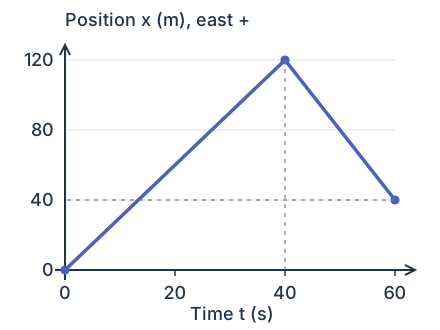
Using $200/60$ for average velocity gives average speed instead: it divides total distance by elapsed time. Do not simply average the two leg velocities either: the legs last different amounts of time.