Motion Graphs: From the Story to the Equation

1. Choose a positive direction and translate the words

Track one object along a straight line in one reference frame throughout the problem. Choose an origin $x=0$ and take right as positive. Time $t$ is measured in seconds, position $x$ in metres, velocity $v$ in metres per second, and acceleration $a$ in metres per second squared.

“Left of the origin”: $x<0$ . This does not tell you the direction of motion.
“Moving left”: $v<0$ . Position is decreasing, even if it is still positive.
“Starts from rest”: the initial velocity is zero. Acceleration can be nonzero.
“Constant velocity”: velocity is unchanged, so $a=0$ throughout that interval.
“Slows down”: the magnitude of velocity decreases. Acceleration opposes velocity; it is not necessarily negative.

Before looking for a formula, mark what changes and when: the start, a change in acceleration, a stop, a reversal, or the finish. An elapsed time begins at the start of your chosen interval, which need not be $t=0$ .

2. Read position: height and slope

On a position–time graph, height gives position at an instant. Slope gives velocity. The plotted curve is not the shape of the road: a curved trace can describe motion along a straight line.

For an interval from $t_i$ to $t_f$ , subscripts i and f mean initial and final. Displacement is $\Delta x=x_f-x_i$ and elapsed time is $\Delta t=t_f-t_i$ . Average velocity is:

$v_{\mathrm{avg}}=\frac{\Delta x}{\Delta t}$

This is the slope of the straight line joining the two endpoints. To estimate velocity at one instant on a smooth curve, draw a tangent: a straight line that follows the curve’s direction at that point. Calculate its slope using two points on the tangent line. This instantaneous velocity can differ from the average over the original interval.

Positive slope: the object moves right. Negative slope: it moves left.
Horizontal segment: position stays fixed; the object is at rest throughout that interval.
Horizontal tangent at one point: velocity is zero at that instant; this does not prove a sustained rest.
Increasing slope magnitude: speed increases. The curve may be rising or falling.

Distance travelled adds the lengths of all parts of the path. Displacement compares only final and initial positions. A round trip has positive distance but can have zero displacement.

3. Read velocity and acceleration: slope and area

On a velocity–time graph, height is velocity; its magnitude $|v|$ is speed. Slope is acceleration. On a straight segment:

$a=\frac{v_f-v_i}{\Delta t}$

The average acceleration over an interval of positive duration is $a_{\mathrm{avg}}=(v_f-v_i)/\Delta t$ , in $\mathrm{m/s^2}$ . It is the slope of the line joining the interval’s endpoints on the velocity–time graph. This ratio remains valid when acceleration changes within the interval; it need not equal the acceleration at every instant.

A horizontal segment at $v=2\,\mathrm{m/s}$ therefore means constant motion, not rest. A downward-sloping line has negative acceleration even while it lies above the time axis.

Signed area under $v(t)$ : it gives $\Delta x$ . A region above zero contributes positively; a region below zero contributes negatively. Its units are $(\mathrm{m/s})\,\mathrm s=\mathrm m$ .
Distance: add the magnitudes of areas separated by velocity’s zero crossings. This is the area under speed $|v|$ .
Signed area under $a(t)$ : it gives the velocity change $\Delta v=v_f-v_i$ , in $\mathrm{m/s}$ . Add that change to $v_i$ to find $v_f$ .

Areas do not supply initial values. A velocity graph alone determines displacements, but not absolute position without $x_i$ . An acceleration graph alone does not determine velocity without $v_i$ .

4. Build three graphs for one journey

Story. A cart starts at $x=0$ . It moves right at $2\,\mathrm{m/s}$ for $3\,\mathrm s$ . From $t=3\,\mathrm s$ to $t=7\,\mathrm s$ , it has constant acceleration $-1\,\mathrm{m/s^2}$ . This acceleration continues when the cart reaches zero velocity.

Split the story before calculating

0 to 3 s: velocity is constant. Acceleration is zero and position rises linearly. The rectangle under velocity gives $\Delta x=2\times3=6\,\mathrm m$ . Thus $x(3)=6\,\mathrm m$ .
3 to 5 s: velocity decreases by $1\,\mathrm{m/s}$ each second. It takes two seconds to change from $2\,\mathrm{m/s}$ to zero. The cart still moves right but slows down.
5 to 7 s: velocity becomes negative and reaches $-2\,\mathrm{m/s}$ . The cart moves left and speeds up. Acceleration did not change at 5 s.

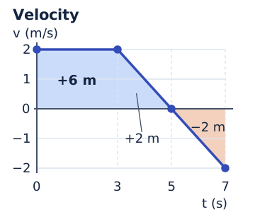
Velocity versus time: 2 m/s from 0 to 3 s, then a straight line from (3 s, 2 m/s) to (7 s, −2 m/s), crossing zero at 5 s. Successive signed areas: +6 m, +2 m, −2 m. — The rectangle and two triangles give displacements. Each triangle has a 2 s base and a 2 m/s height, so its area magnitude is 2 m.

Total displacement and total distance are therefore:

$\Delta x=6+2-2=6\,\mathrm m$

$D=6+2+2=10\,\mathrm m$

Here $D$ means distance travelled. Position reaches $8\,\mathrm m$ at 5 s, then returns to $6\,\mathrm m$ at 7 s. The cart returns to its 3 s position, not to the origin.

Position versus time: a straight segment from (0 s, 0 m) to (3 s, 6 m), followed by a concave-down parabola through (5 s, 8 m) and (7 s, 6 m). The tangent is horizontal at 5 s. — From 3 to 5 s, position rises with a shrinking positive slope. From 5 to 7 s, it falls with an increasingly negative slope. The curve is concave down throughout the second phase.

Acceleration versus time: 0 m/s² before 3 s and −1 m/s² after 3 s, through 7 s. Two open circles at 3 s indicate that instantaneous acceleration at the switch is undefined in this model. — The signed area under the acceleration–time graph from 3 to 7 s is −4 m/s: velocity changes from +2 to −2 m/s. The idealized switch at 3 s creates no jump in position or velocity. Acceleration at that exact instant is undefined.

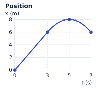
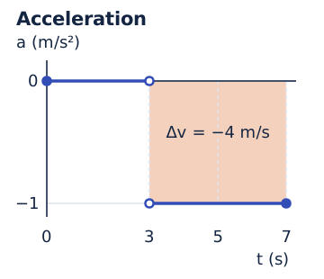
At $t=5\,\mathrm s$ , $v=0$ but $a=-1\,\mathrm{m/s^2}$ . The velocity graph has zero height while its slope remains negative. The sign change in velocity establishes the reversal; zero velocity alone is not enough.

Show the functions used to plot the graphs

To reproduce these numerical plots, enter $t$ in seconds; the formulas return $x$ in metres and $v$ in metres per second. For $0\le t\le3$ :

$x=2t$

$v=2$

For $3\le t\le7$ , set $\tau=t-3$ , the elapsed time in seconds since the switch:

$x=6+2\tau-\frac12\tau^2$

$v=2-\tau$

The position and velocity formulas agree at 3 s. These functions do not specify motion after 7 s.

5. Choose an equation on a valid interval

The four relationships below assume constant acceleration over the chosen interval. They include $a=0$ . In our journey, separate 0–3 s from 3–7 s. These equations do not require another split at 5 s because acceleration stays constant there; the 5 s split is needed for distance.

For each interval, list $v_i$ , $v_f$ , $a$ , $\Delta t$ and $\Delta x$ . Mark the knowns and your target. Prefer a relationship containing only one unknown.

Without using displacement

$v_f=v_i+a\Delta t$

Links velocities, acceleration and elapsed time. Useful for finding when velocity reaches zero.

Without using final velocity

$\Delta x=v_i\Delta t+\frac12a\Delta t^2$

Gives displacement from initial velocity, acceleration and elapsed time.

Without using elapsed time

$v_f^2=v_i^2+2a\Delta x$

Links velocities to displacement. Squaring loses the sign: choose velocity’s direction from the motion.

Without explicitly using acceleration

$\Delta x=\frac{v_i+v_f}{2}\Delta t$

Gives signed area under a straight velocity line. Averaging endpoint velocities is not a general method when acceleration varies.

The absence of acceleration in the data does not make it constant. If velocity is curved or acceleration changes, use available areas, split into justified phases, or use a variable-acceleration model. Do not simply replace $a$ by its average in every equation.

6. Solve a stop without extending the braking model

A cart moves at $12\,\mathrm{m/s}$ and brakes at constant acceleration $-3\,\mathrm{m/s^2}$ until it stops. It then remains stationary. How far does it travel while braking?

Choose, calculate, check

Take the initial direction as positive. We know $v_i=12\,\mathrm{m/s}$ , $v_f=0$ and $a=-3\,\mathrm{m/s^2}$ . Elapsed time is unknown and unnecessary for displacement: choose the no-time relationship.

$\Delta x=\frac{v_f^2-v_i^2}{2a}$

$\Delta x=24\,\mathrm m$

The numerator and denominator are both negative, so displacement is positive. Because the cart does not reverse before stopping, distance is also 24 m.

Check using stopping time and the triangular area under velocity:

$\Delta t=\frac{v_f-v_i}{a}=4\,\mathrm s$

$D=\frac12(4)(12)=24\,\mathrm m$

After these 4 s, the story specifies rest: $v=0$ and $a=0$ . Extending acceleration at −3 m/s² would make the cart reverse and would describe a different motion.

7. Try six progressively harder questions

Try each question before opening its hint. Label axes and units in your sketches, mark important times, and justify each phase change.

1. Does negative position mean leftward motion?

A position–time graph is a straight line from $(0\,\mathrm s,-4\,\mathrm m)$ to $(3\,\mathrm s,2\,\mathrm m)$ . Find velocity, acceleration, displacement and distance.

Show a hint

Slope uses a position difference; a straight line has constant slope.

Show the explained solution

Position increases: the object moves right even while it is left of the origin.

$\Delta x=2-(-4)=6\,\mathrm m$

$v=6/3=2\,\mathrm{m/s}$

Velocity is constant, so $a=0$ . There is no reversal: $D=6\,\mathrm m$ . The velocity graph is horizontal at +2 m/s; the acceleration graph is horizontal at zero.

2. Cross zero on a velocity graph

Velocity rises linearly from $-3\,\mathrm{m/s}$ to $+1\,\mathrm{m/s}$ over 4 s, starting at $t=0$ . Find acceleration, reversal time, displacement and distance. Describe the position graph.

Show a hint

Velocity reaches zero before the end. Separate the two triangles when finding distance.

Show the explained solution

$a=\frac{1-(-3)}{4}=1\,\mathrm{m/s^2}$

It takes 3 s to change from −3 m/s to zero. Before then, the object moves left and slows down; afterwards, it moves right and speeds up.

The negative triangle has signed area −4.5 m and the positive triangle has area +0.5 m.

$\Delta x=-4.5+0.5=-4\,\mathrm m$

$D=4.5+0.5=5\,\mathrm m$

Position is a concave-up parabola with a minimum at 3 s. Its absolute height is unknown without initial position. Negative displacement is consistent with positive final velocity.

3. Reach the same position twice

Return to the cart in section 4. At what times is it at $x=7.5\,\mathrm m$ ? What is its velocity at each time?

Show a hint

Position exceeds 6 m only in the second phase. Use elapsed time since 3 s and retain both roots if they fall within that phase.

Show the explained solution

In the numerical graph formula, $\tau=t-3$ is in seconds. The equation becomes:

$7.5=6+2\tau-\frac12\tau^2$

$\tau^2-4\tau+3=0$

$(\tau-1)(\tau-3)=0$

Elapsed times of 1 s and 3 s both lie within the 4 s phase. They give $t=4\,\mathrm s$ and $t=6\,\mathrm s$ . Using $v=2-\tau$ , velocities are $+1\,\mathrm{m/s}$ and $-1\,\mathrm{m/s}$ , respectively. The cart passes the same point on its outward and return legs. Automatically rejecting the second root would discard a real event.

4. Change the model after a stop

An object moves at 8 m/s, brakes uniformly at −2 m/s² until it stops, then remains at rest for 3 s. Find total distance, total elapsed time and average velocity over the full motion.

Show a hint

First find braking time. The rest phase increases total elapsed time without adding displacement.

Show the explained solution

$\Delta t_{\mathrm b}=\frac{0-8}{-2}=4\,\mathrm s$

Here subscript b denotes braking. The triangle under velocity has a 4 s base and an 8 m/s height:

$\Delta x=\frac12(4)(8)=16\,\mathrm m$

The object does not reverse. Thus $D=16\,\mathrm m$ and total elapsed time is $7\,\mathrm s$ .

$v_{\mathrm{avg}}=\frac{16}{7}\,\mathrm{m/s}$

This is about 2.29 m/s. Velocity falls to zero at 4 s, then stays at zero until 7 s. Position rises, flattens at the stop, then stays horizontal. The endpoint-velocity average, 4 m/s, does not apply to the whole motion: acceleration changes at the stop.

5. Same endpoint velocities, same displacement?

Two objects start from rest at the same position. A accelerates uniformly, reaching 8 m/s at 4 s. B stays at rest for 2 s, then accelerates uniformly, also reaching 8 m/s at 4 s. Compare their average accelerations and displacements from 0 to 4 s.

Show a hint

Their velocity changes are equal. Do the triangles under their velocity graphs have equal bases?

Show the explained solution

Both average accelerations are $8/4=2\,\mathrm{m/s^2}$ . For A, that acceleration is constant. For B, acceleration is zero for 2 s, then $4\,\mathrm{m/s^2}$ for 2 s.

$\Delta x_A=\frac12(4)(8)=16\,\mathrm m$

$\Delta x_B=\frac12(2)(8)=8\,\mathrm m$

Average acceleration fixes the total velocity change, not how that change is distributed in time. Treating B as if it had constant acceleration of 2 m/s² would give the wrong displacement. Its delayed start reduces the area under velocity.

6. Combine a delay and braking

A test cart moves at 20 m/s. After a signal, its controller maintains that velocity for 0.8 s, then applies acceleration of −5 m/s² until the cart stops. A marker is 60 m ahead of the cart’s position at the signal. Does the cart stop before the marker? How long after the signal?

Show a hint

There are two phases. Braking begins at a new position but with the same velocity as during the delay.

Show the explained solution

Choose the signal position as the origin and the initial direction as positive. During the delay, $a=0$ and velocity stays at 20 m/s:

$\Delta x_1=20(0.8)=16\,\mathrm m$

For braking, $v_i=20\,\mathrm{m/s}$ and $v_f=0$ . The no-time relationship gives that phase’s displacement:

$\Delta x_2=\frac{0^2-20^2}{2(-5)}$

$\Delta x_2=40\,\mathrm m$

Subscripts 1 and 2 denote the delay and braking. Total displacement is $16+40=56\,\mathrm m$ . There is no reversal, so this is also distance. The cart stops 4 m before the marker.

$\Delta t_2=\frac{0-20}{-5}=4\,\mathrm s$

$\Delta t=0.8+4=4.8\,\mathrm s$

On the velocity graph, a rectangle with base 0.8 s precedes a triangle with base 4 s. One constant acceleration over the entire 4.8 s does not represent this motion.

Optional extension: relative velocity and river crossings

Allow 20–25 minutes. The main motion-graph lesson stands on its own. This extension needs signed components, Pythagoras and inverse trigonometric functions in degree mode. If components are unfamiliar, review vector components and direction: that lesson uses forces, but the component addition method also works for velocities.

Name the object and the observer

A reference frame is a choice of origin, axes and clock used to measure motion. A passenger can be at rest in a train's frame and moving in the ground's frame. Neither velocity is meaningful without its observer. Here all axes remain parallel and do not rotate; frames move at constant velocity relative to one another, and speeds are far below the speed of light. We use ordinary, or Galilean, velocity addition.

Write $\mathbf v_{A/B}$ for the velocity of object A relative to observer B. The slash means “relative to”, not division. G denotes the ground. Take east as positive x and north as positive y, with components in the order $(v_x,v_y)$ , in m/s. A bold symbol is a vector; $|\mathbf v|$ is its nonnegative speed.

\mathbf v_{A/G}=\mathbf v_{A/B}+\mathbf v_{B/G}

\mathbf v_{A/B}=\mathbf v_{A/G}-\mathbf v_{B/G}

Subtract the observer's velocity from the object's velocity, component by component. Reversing object and observer reverses the vector:

\mathbf v_{B/A}=-\mathbf v_{A/B}.

This follows from subtracting their ground positions at the same time: the change in A's position relative to B is the change in A's ground position minus the change in B's. For a head-to-tail diagram, draw the object's ground velocity followed by the negative of the observer's ground velocity. The resultant points from the starting tail to the final tip. A velocity triangle is not a map of the objects' locations.

Worked example 1: what does a moving observer measure?

On separate paths, skater A travels east at 6 m/s and skater B travels north at 8 m/s, both measured from the ground. Their velocities are constant. Find A's velocity relative to B, and then B's relative to A.

\begin{aligned}\mathbf v_{A/G}&=(6,0)\,\mathrm{m/s},\\\mathbf v_{B/G}&=(0,8)\,\mathrm{m/s},\\\mathbf v_{A/B}&=(6,0)-(0,8)\\&=(6,-8)\,\mathrm{m/s}.\end{aligned}

To B, A moves east and south. The relative speed and the acute angle south of east are:

\begin{aligned}|\mathbf v_{A/B}|&=\sqrt{6^2+(-8)^2}=10\,\mathrm{m/s},\\\alpha&=\arctan(8/6)\approx53.13^\circ.\end{aligned}

The answer is 10 m/s, 53.13° south of east. B's velocity relative to A is:

\mathbf v_{B/A}=(-6,8)\,\mathrm{m/s}.

It has the same speed, 53.13° north of west. Check: adding B's ground velocity back to A's relative velocity gives $(6,-8)+(0,8)=(6,0)\,\mathrm{m/s}$ . Subtracting the speeds, 6 − 8, would discard their perpendicular directions. These velocities alone do not tell us whether the skaters meet: their initial positions are also needed.

Worked example 2: cross fastest, or land directly opposite?

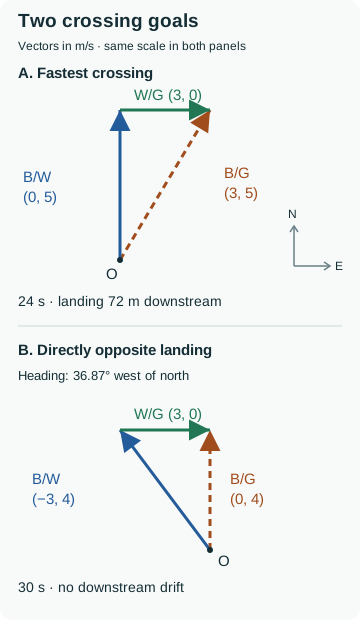
A straight river is 120 m wide from its south bank to its north bank. Its uniform current flows east at 3 m/s relative to the shore. A boat maintains a speed of 5 m/s relative to the water. Ignore start-up and landing time. Keep each chosen heading constant. B denotes the boat, W the water and G the shore, treated as the ground frame.

\mathbf v_{B/G}=\mathbf v_{B/W}+\mathbf v_{W/G}

The current has no northward component. Crossing time therefore uses the northward shore component, not total shore speed. Let d be the river width and let $v_{B/G,y}>0$ be that component:

t=\frac{d}{v_{B/G,y}}.

A. Reach any point on the opposite bank in the least time

Assume any downstream landing point is allowed. Point the boat due north relative to the water. This puts all 5 m/s of its water-relative speed into crossing; any angled heading gives a smaller northward component.

\begin{aligned}\mathbf v_{B/W}&=(0,5)\,\mathrm{m/s},\\\mathbf v_{W/G}&=(3,0)\,\mathrm{m/s},\\\mathbf v_{B/G}&=(3,5)\,\mathrm{m/s}.\end{aligned}

\begin{aligned}t_{\min}&=120/5=24\,\mathrm s,\\\Delta x&=3(24)=72\,\mathrm m.\end{aligned}

The boat lands 72 m downstream of the directly opposite point. Its shore speed is $\sqrt{34}\,\mathrm{m/s}\approx5.83\,\mathrm{m/s}$ , and its track is $\arctan(3/5)\approx30.96^\circ$ east of north. The heading is due north; the shore track is tilted downstream. Dividing 120 m by 5.83 m/s would mix a perpendicular width with a diagonal speed.

B. Land directly opposite the starting point

Now require zero eastward shore velocity. The boat must supply a water-relative x component of −3 m/s (westward) to cancel the current. Its total water-relative speed must still be 5 m/s.

\begin{aligned}v_{B/W,x}&=-3\,\mathrm{m/s},\\v_{B/W,y}&=\sqrt{5^2-3^2}=4\,\mathrm{m/s},\\\mathbf v_{B/G}&=(-3,4)+(3,0)\\&=(0,4)\,\mathrm{m/s}.\end{aligned}

The upstream heading angle, measured west of north, and the crossing time are:

\begin{aligned}\theta&=\arcsin(3/5)\approx36.87^\circ,\\t&=120/4=30\,\mathrm s.\end{aligned}

Check: $\sqrt{(-3)^2+4^2}=5\,\mathrm{m/s}$ , and the eastward components cancel. Landing directly opposite takes 6 s longer than reaching the bank anywhere.

Two head-to-tail velocity triangles use 30 drawing units per metre per second. For the fastest crossing, boat through water (0, 5) plus current (3, 0) gives shore velocity (3, 5). For a directly opposite landing, boat through water (−3, 4) plus current (3, 0) gives shore velocity (0, 4). — Both velocity triangles use the same scale. Solid arrows add head to tail; the dashed arrow is the shore velocity. These are velocities, not distances across the river.

Check feasibility before using an inverse sine

For a river of width d, boat speed u relative to the water and current speed c parallel to the bank, assume $d>0$ , $u>0$ and $c\ge0$ . With no restriction on downstream landing, the fastest crossing is $t_{\min}=d/u$ , with drift $cd/u$ . For a directly opposite landing, the required upstream component has magnitude c:

\sin\theta=\frac{c}{u},\qquad v_{B/G,y}=\sqrt{u^2-c^2}.

When $c<u$ : a finite directly opposite crossing is possible, with $t=d/\sqrt{u^2-c^2}$ .
When $c=u$ : cancelling the current uses the entire boat speed. The boat points straight upstream, its shore velocity is zero, and it makes no progress across. There is no finite directly opposite crossing.
When $c>u$ : the boat cannot cancel the current; an inverse sine of c/u has no real value. A directly opposite crossing is impossible in this model.

A strong current does not prevent every crossing in this ideal model: pointing north still gives positive northward speed while drifting downstream. A real river may have hazards or inaccessible landing points; these equations are a classroom model, not boating advice.

Try four progressively harder questions

Use the frame labels explicitly. All given velocities and river currents stay constant. Try a question before opening its hint and worked solution.

1. Keep the sign in one dimension

A train T moves east at 18 m/s relative to the ground G. Passenger P walks west at 1.5 m/s relative to the train. Find the passenger's ground velocity and the ground's velocity relative to the passenger.

Show hint 1

Use east as positive. The walking velocity is negative in the train frame. Add velocities with the common frame T in the middle.

Show worked solution 1

\begin{aligned}v_{P/G}&=v_{P/T}+v_{T/G}\\&=-1.5+18=16.5\,\mathrm{m/s},\\v_{G/P}&=-16.5\,\mathrm{m/s}.\end{aligned}

The passenger moves east relative to the ground at 16.5 m/s, despite walking west inside the train. To the passenger, the ground moves west at 16.5 m/s. Check: $16.5-18=-1.5\,\mathrm{m/s}$ recovers the stated walking velocity.

2. Subtract two component pairs

Cyclist A has ground velocity (4, 3) m/s and cyclist B has ground velocity (−2, 1) m/s. Find A's velocity relative to B: components, speed and direction. Then reverse the observer.

Show hint 2

Subtract B's x component and B's y component separately. Predict the quadrant before using inverse tangent.

Show worked solution 2

\begin{aligned}\mathbf v_{A/B}&=(4,3)-(-2,1)\\&=(6,2)\,\mathrm{m/s},\\|\mathbf v_{A/B}|&=\sqrt{6^2+2^2}=\sqrt{40}\,\mathrm{m/s}\\&\approx6.32\,\mathrm{m/s},\\\alpha&=\arctan(2/6)\approx18.43^\circ.\end{aligned}

A moves 18.43° north of east relative to B. Reversing the observer gives $\mathbf v_{B/A}=(-6,-2)\,\mathrm{m/s}$ , the same speed at 18.43° south of west. Check: $(6,2)+(-2,1)=(4,3)\,\mathrm{m/s}$ . A relative speed alone cannot determine an encounter time without initial positions.

3. Find the fastest crossing and its landing point

A boat crosses an 80 m wide river from its south bank to its north bank. The current flows east at 3 m/s. A boat's speed relative to the water is 4 m/s. Any opposite-bank landing point is allowed. Find the fastest heading, crossing time, drift, shore speed and shore-track direction.

Show hint 3

Maximize the northward component. Multiply the current speed by the crossing time to obtain downstream displacement.

Show worked solution 3

\begin{aligned}\mathbf v_{B/W}&=(0,4)\,\mathrm{m/s},\\\mathbf v_{B/G}&=(0,4)+(3,0)\\&=(3,4)\,\mathrm{m/s},\\t_{\min}&=80/4=20\,\mathrm s,\\\Delta x&=3(20)=60\,\mathrm m,\\|\mathbf v_{B/G}|&=\sqrt{3^2+4^2}=5\,\mathrm{m/s}.\end{aligned}

Head due north relative to the water. The shore track is $\arctan(3/4)\approx36.87^\circ$ east of north, and the boat lands 60 m downstream. Check: the displacement is (60, 80) m, with length 100 m; $100/5=20\,\mathrm s$ . Using $80/5=16\,\mathrm s$ would incorrectly use the width as the diagonal distance.

4. Test a directly opposite crossing and its limits

A boat crosses a 60 m wide river from its south bank to its north bank. The current flows east; the boat maintains 2 m/s relative to the water. Can it land directly opposite when the current is (a) 1.2 m/s, (b) 2 m/s, or (c) 2.5 m/s? For (a), find the heading and time. For (c), explain whether a crossing to some downstream point is still possible.

Show hint 4

First compare current speed with boat speed. To land directly opposite, cancel the current and check that a strictly positive northward component remains.

Show worked solution 4

(a) Since 1.2 is less than 2, cancel the current using a water-relative x component of −1.2 m/s (westward):

\begin{aligned}v_{B/W,y}&=\sqrt{2^2-1.2^2}=1.6\,\mathrm{m/s},\\\mathbf v_{B/G}&=(-1.2,1.6)+(1.2,0)\\&=(0,1.6)\,\mathrm{m/s},\\\theta&=\arcsin(1.2/2)\approx36.87^\circ,\\t&=60/1.6=37.5\,\mathrm s.\end{aligned}

Head 36.87° west of north. Check: $\sqrt{1.2^2+1.6^2}=2\,\mathrm{m/s}$ .

(b) An x component of −2 m/s (westward) leaves zero northward component. The shore velocity is zero when the current is cancelled. A 90° upstream heading does not carry the boat across; there is no finite crossing time.

(c) A required x component of −2.5 m/s (westward) exceeds the boat's total water-relative speed. A directly opposite landing is impossible. However, heading due north gives:

\begin{aligned}\mathbf v_{B/G}&=(2.5,2)\,\mathrm{m/s},\\t&=60/2=30\,\mathrm s,\\\Delta x&=2.5(30)=75\,\mathrm m.\end{aligned}

It can reach a point 75 m downstream in this ideal model if that landing point is allowed. The failure is the directly opposite target, not northward motion itself.

Keep the models and course connections precise

Before solving, name both frames, choose common axes, write the vector equation and state the landing constraint. Check the component that determines crossing time and whether the required heading is physically possible. The person walking in a freely moving boat is a different setup: its unknown boat motion is obtained from a system balance. Here the water-relative boat speed and current are given.

The relative-motion and two-dimensional vector work directly connects to Ontario SPH4U, expectation B2.2, printed page 198. This is a topic connection, not coverage of the whole course. The university links elsewhere in this lesson establish broader kinematics connections; they do not by themselves verify that every course assesses river crossings. Check your own outline. See also OpenStax, Relative Motion in One and Two Dimensions for the frame convention. The examples, numbers, diagrams and exercises here are original.

Optional calculus transfer: the same rule, a different quantity

Prerequisites: derivatives of polynomials and definite integrals. If your course uses algebraic motion graphs only, the six questions above work on their own.

Take right as positive. Let $t$ be numerical time in seconds, with $0\le t\le6$ . These are two independent cart scenarios. Position locates a cart; displacement is final minus initial position. Distance adds all lengths travelled, regardless of direction.

Cart A: the rule gives velocity

Velocity $v(t)$ is in m/s and position $x(t)$ is in metres:

$v(t)=5-0.4t+0.1t^2$

Initially, $x(0)=-2\,\mathrm m$ . Find acceleration $a(2)$ , position $x(6)$ , and total distance from 0 to 6 s. Is the cart at rest when acceleration is zero? Write and justify each derivative or definite integral; a numerical answer alone is not enough.

Show a hint for Cart A

Differentiate velocity for acceleration. Integrate velocity for displacement, then add initial position. Check velocity’s sign before finding distance.

Show Cart A’s explained solution

Acceleration $a(t)=v'(t)$ , in m/s², is:

$a(t)=-0.4+0.2t$

Thus $a(2)=0\,\mathrm{m/s^2}$ , but $v(2)=4.6\,\mathrm{m/s}$ : the cart is moving right. Acceleration varies, so constant-acceleration formulas do not apply over the whole interval.

Signed area under velocity gives displacement:

$\Delta x=\int_0^6 v(t)\,dt$

$\Delta x=\left[5t-0.2t^2+\frac{t^3}{30}\right]_0^6$

$\Delta x=30\,\mathrm m$

Therefore $x(6)=-2+30=28\,\mathrm m$ . Throughout the interval,

$v(t)=0.1(t-2)^2+4.6>0$

so the cart never reverses and distance is also 30 m. Using the constant value $v(0)=5\,\mathrm{m/s}$ for six seconds happens to give 30 m, but wrongly treats the changing velocity as constant.

Separate retry, Cart B: the rule gives position

The same polynomial now gives position $p(t)$ , in metres:

$p(t)=5-0.4t+0.1t^2$

This cart starts at $p(0)=5\,\mathrm m$ . Find its velocity and acceleration at 2 s, then its displacement and distance from 0 to 6 s. Justify the operations you choose.

Show a hint for Cart B

Differentiate position once for velocity and twice for acceleration. Check whether velocity changes sign before adding lengths travelled.

Show Cart B’s explained solution

Velocity is $p'(t)=-0.4+0.2t$ , in m/s; acceleration is $p''(t)=0.2$ , in m/s². Hence $p'(2)=0\,\mathrm{m/s}$ and $p''(2)=0.2\,\mathrm{m/s^2}$ .

Velocity changes from negative to positive at 2 s. The positions at 0, 2 and 6 s are 5, 4.6 and 6.2 m. Displacement is $6.2-5=1.2\,\mathrm m$ ; distance is $0.4+1.6=2.0\,\mathrm m$ . Here the given function is position: its meaning and units change the required operation.

8. Check the model and result efficiently

Reference direction: does every signed value match your chosen positive direction?
Interval: is acceleration constant throughout the phase you used? Does elapsed time start at the correct instant?
Graphs: does position’s slope match velocity? Does velocity’s slope match acceleration?
Areas: did you add signed areas for displacement and their magnitudes for distance?
Events: does the stop last, or does velocity change sign? Does each calculated root lie inside the model’s phase?
Units and meaning: are the units correct? Distance cannot be smaller than the magnitude of displacement.

To work efficiently, first write one short line per phase: elapsed time, initial velocity, acceleration and target. This prevents choosing a formula with data mixed from two different phases.

When the missing step is finding acceleration from interactions, continue with free-body diagrams and friction. For choosing other mechanics balances, see work, energy and momentum.

9. References and course connection

The official descriptions of Concordia PHYS 204 and McGill PHYS 101 include kinematics. These establish topic connections; they do not make the courses equivalent or imply that this lesson covers their full content. The explanations, data, figures and questions were created for this resource.

Motion Graphs: From the Story to the Equation

1. Choose a positive direction and translate the words

2. Read position: height and slope

3. Read velocity and acceleration: slope and area

4. Build three graphs for one journey

Split the story before calculating

5. Choose an equation on a valid interval

Without using displacement

Without using final velocity

Without using elapsed time

Without explicitly using acceleration

6. Solve a stop without extending the braking model

Choose, calculate, check

7. Try six progressively harder questions

1. Does negative position mean leftward motion?

2. Cross zero on a velocity graph

3. Reach the same position twice

4. Change the model after a stop

5. Same endpoint velocities, same displacement?

6. Combine a delay and braking

Optional extension: relative velocity and river crossings

Name the object and the observer

Worked example 1: what does a moving observer measure?

Worked example 2: cross fastest, or land directly opposite?

A. Reach any point on the opposite bank in the least time

B. Land directly opposite the starting point

Check feasibility before using an inverse sine

Try four progressively harder questions

1. Keep the sign in one dimension

2. Subtract two component pairs

3. Find the fastest crossing and its landing point

4. Test a directly opposite crossing and its limits

Keep the models and course connections precise

Optional calculus transfer: the same rule, a different quantity

Cart A: the rule gives velocity

Separate retry, Cart B: the rule gives position

8. Check the model and result efficiently

9. References and course connection

Useful for

Work on the step you’re missing.

Free study guides and practice

Free-Body Diagrams and Friction: From Forces to Equations

Work, Energy or Momentum: Choose the Method

Projectile motion with different launch and landing heights