How to Choose an Integration Method

1. Read the structure before choosing a formula

Knowing integration formulas does not always tell you how to begin. A useful first question is: what change would make this integrand easier to integrate? You might rewrite its algebra, rename a composite expression, or trade one integral for a simpler one.

This lesson develops that judgment through substitution, integration by parts, partial fractions, and trigonometric substitution. You should know basic antiderivatives and the chain and product rules. By the end, aim to explain your first move, recognize when it is unhelpful, and check your result.

In the notation below, $x$ is the variable of integration, $dx$ identifies that variable, and the integrand is the expression being integrated. An antiderivative is a function whose derivative equals the integrand. The symbol $C$ is an arbitrary real constant: adding a constant does not change a derivative. The number $e\approx2.718$ is the base of the natural exponential, and $\ln$ is its inverse logarithm.

Compare these almost identical integrals:

$$\int x e^{x^2}\,dx \qquad\text{and}\qquad \int x e^{2x}\,dx$$

Both contain a product. In the first, the derivative of the exponent is $2x$, so the outside $x$ supplies the needed derivative, up to a constant. In the second, the exponent’s derivative is just $2$; the outside $x$ remains. That small change makes substitution natural for the first and integration by parts useful for the second.

Route through the lesson: simplify first → substitution → by parts → partial fractions → combine and check → trigonometric substitution → practice. Read the worked examples in order, then cover the solutions while you practise.

2. Simplify before reaching for a technique

An integral that looks like a quotient may need only division or cancellation. For example,

$$\begin{aligned}&\int\frac{x^2+1}{x}\,dx\\&=\int\left(x+\frac1x\right)dx\\&=\frac{x^2}{2}+\ln|x|+C,\qquad x\ne0.\end{aligned}$$

The logarithm appears because the power rule excludes exponent $-1$. There is no need to introduce another method. Similarly, expanding a short polynomial product can be easier than applying integration by parts. Keep a compact power such as $(x^2+4)^8$ intact when its inside derivative is nearby.

If this algebra is the obstacle, revisit Before calculus algebra skills. Here, we will focus on what the algebra reveals about integration.

3. Substitution reverses the chain rule

Let $f$ be a function and let $F$ be one of its antiderivatives, so $F^{\prime}(u)=f(u)$; a prime denotes differentiation. Let $g(x)$ be a differentiable inner function and use $u$ as a name for its output. The chain rule says

$$\frac{d}{dx}F(g(x))=f(g(x))g'(x).$$

Reading this backward explains substitution: when an integrand contains $f(g(x))$ together with $g'(x)$, setting $u=g(x)$ packages those pieces into $f(u)\,du$. The differential $du=g'(x)\,dx$ records the change of variable; it is not an optional decoration.

Test the whole substitution

For $\int xe^{x^2}\,dx$, $u=x^2$ gives $\frac12\int e^u\,du$, hence $\frac12e^{x^2}+C$. But removing the outside $x$ changes the problem: with $\int e^{x^2}\,dx$, the same substitution does not leave $\int e^u\,du$. You cannot discard the factor needed to replace $dx$.

Checkpoint: after substituting, have you rewritten every variable and the differential consistently, and is the new integral easier? A visible inside derivative is a strong clue, not a requirement for every useful substitution. Sometimes you must also express a leftover $x$ in terms of $u$.

4. See why the differential and bounds matter

Consider a definite integral with $u=x^2+1$ and $du=2x\,dx$. When $x=0$, $u=1$; when $x=1$, $u=2$:

$$\int_0^1\frac{2x}{x^2+1}\,dx=\int_1^2\frac1u\,du=\ln2.$$

The graphs below have different shapes and horizontal ranges, but equal shaded areas. Substitution changes both the function description and the horizontal measure.

The symbol $\Delta x$ denotes a small change in $x$; $\Delta u$ is the corresponding change in $u$. For a sufficiently narrow strip, $\Delta u\approx2x\,\Delta x$; in the limit, $du=2x\,dx$. The original height $2x/(x^2+1)$ and the new height $1/u$ describe the same accumulated quantity when paired with the appropriate width. Merely changing the function’s name would miss that compensation.

There are two consistent ways to finish a definite integral:

• Change to $u$ throughout, including the bounds, as above
• Find an antiderivative, substitute back to $x$, and then use the original $x$ bounds

Do not combine a $u$ antiderivative with unchanged $x$ bounds. Do not append $+C$ to the final numerical value: the constant cancels when you subtract endpoint values.

Quick comparison: $\int 2x/(x^2+1)\,dx$ suggests a logarithm. The similar-looking $\int 1/(x^2+1)\,dx$ is the standard arctangent integral. The numerator changes which derivative pattern is present.

5. Integration by parts reverses the product rule

For this method, $u$ and $v$ denote differentiable functions of $x$; they are new choices, unrelated to the substitution variable in the previous section. Their differentials are $du=u^{\prime}(x)\,dx$ and $dv=v^{\prime}(x)\,dx$. The product rule gives $d(uv)=u\,dv+v\,du$. Integrate and rearrange:

$$\int u\,dv=uv-\int v\,du.$$

This exchanges one integral for another. Choose $u$ so that differentiating it helps, and choose $dv$ so you can actually find $v$. Then inspect the remaining integral before committing to a long calculation.

A product can be hidden

For $\int\ln x\,dx$, write the integrand as $\ln x\cdot1$, with $x>0$. Choose $u=\ln x$ and $dv=dx$:

$$\begin{aligned}&\int\ln x\,dx\\&=x\ln x-\int x\frac1x\,dx\\&=x\ln x-x+C.\end{aligned}$$

The gain comes from cancellation in $v\,du$, even though $1/x$ may not look simpler on its own. This is why a rule such as “differentiate the logarithm first” is a useful suggestion, not a proof that a choice will work.

Common misconception: integrating a product does not mean multiplying its two antiderivatives. For example, $\int x\cdot x\,dx=x^3/3+C$, whereas $(x^2/2)(x^2/2)=x^4/4$ differentiates to $x^3$, not $x^2$.

6. Partial-fraction decomposition reverses combining fractions

Partial fractions is an algebraic rewrite of a rational function, a ratio of polynomials. It reveals simpler terms whose antiderivatives you already know. Before decomposing, divide if the numerator’s degree is at least the denominator’s, and check whether cancellation or a direct substitution already finishes the job.

A denominator alone does not choose the method

For $\int(2x+3)/(x^2+3x+2)\,dx$, the numerator is exactly the denominator’s derivative. Substitution immediately gives $\ln|x^2+3x+2|+C$. Partial fractions also works, giving $\ln|x+1|+\ln|x+2|+C$. These expressions agree wherever the denominator is nonzero.

The worked example’s numerator, $3x+5$, is not a constant multiple of $2x+3$. Direct substitution therefore does not remove all the work. You can split off a derivative-matching part, but a remainder still needs attention.

Know the next cases

In the next forms, $A$, $B$, and $D$ are unknown real coefficients to determine by matching numerators; $D$ avoids confusing a coefficient with the integration constant $C$. Repeated factors need all their powers: a denominator $x(x+1)^2$ requires the form

$$\frac{A}{x}+\frac{B}{x+1}+\frac{D}{(x+1)^2}.$$

An irreducible quadratic cannot be factored into real linear factors. Such a quadratic, for example $x^2+1$ needs a possible linear numerator $(Ax+B)/(x^2+1)$. It can lead to both logarithms and arctangents. Stopping because a denominator does not split into real linear factors misses these cases.

For example, splitting the numerator exposes both familiar patterns:

$$\begin{aligned}&\int\frac{2x+3}{x^2+1}\,dx\\&=\ln(x^2+1)\\&\quad+3\arctan x+C.\end{aligned}$$

7. Combine methods and check the domain

Methods often work in sequence. In $\int x^3e^{x^2}\,dx$, write $x^3\,dx=x^2(x\,dx)$. Substitution gives $u=x^2$, then by parts handles $ue^u$:

$$\begin{aligned}&\int x^3e^{x^2}\,dx\\&=\frac12\int ue^u\,du\\&=\frac12(u-1)e^u+C\\&=\frac12(x^2-1)e^{x^2}+C.\end{aligned}$$

The useful question after substitution is again: what structure does the new integral have?

An antiderivative belongs on an interval

For the partial-fractions example, the integrand is undefined at $-2$ and $-1$. Its antiderivative formula works on each of the three intervals separated by those points. The constants on different intervals need not be equal.

Do not use endpoint subtraction across a singularity without checking the relevant improper integrals. For example, $\int_{-1}^{1}1/x\,dx$ diverges as an ordinary improper integral; substituting endpoints into $\ln|x|$ and reporting zero is invalid.

A practical stopping and checking routine

Differentiate your candidate answer and simplify toward the original integrand. Check signs, constant factors, and the interval where both expressions are valid. A numerical spot-check may catch a mistake, but it cannot prove an identity or convergence.

If a trial leaves a harder integral, reconsider it. Trigonometric identities, trigonometric substitution, repeated by parts, or other tools may be appropriate. Some continuous functions, including $e^{x^2}$, have antiderivatives that cannot be expressed using elementary functions: finite combinations of the usual algebraic, exponential, logarithmic, trigonometric, and inverse-trigonometric functions. Their definite integrals over finite intervals can still be approximated numerically. Failure of one method is not proof that no elementary antiderivative exists.

When a quadratic radical remains, compare the sine, tangent and secant substitutions below. Match the identity, choose an angle interval and check its sign before calculating.

8. Trigonometric substitution: match the radical and its sign

A trigonometric substitution can turn a quadratic radical into a familiar trigonometric expression. First check whether an ordinary substitution already helps: an accompanying factor $x\,dx$ may make $u=x^2+a^2$ sufficient. Otherwise, compare the three forms below. Let $a>0$ be a fixed constant, and measure the new angle $\theta$ in radians. Here $\sec\theta=1/\cos\theta$.

Three radicals, three identities

A constant square minus a variable square: for $\sqrt{a^2-x^2}$, choose sine because $1-\sin^2\theta=\cos^2\theta$.

$$\begin{gathered}x=a\sin\theta,\\dx=a\cos\theta\,d\theta,\\-\frac\pi2\le\theta\le\frac\pi2,\\\sqrt{a^2-x^2}=a|\cos\theta|\\=a\cos\theta.\end{gathered}$$

This interval covers $-a\le x\le a$ and gives $\cos\theta\ge0$. If the radical is in a denominator, exclude $x=\pm a$ and use the open angle interval. For a complete sine example and the return to $x$, see Question 6(b): sine substitution for a difference of squares.

A sum of squares: for $\sqrt{a^2+x^2}$, choose tangent because $1+\tan^2\theta=\sec^2\theta$.

$$\begin{gathered}x=a\tan\theta,\\dx=a\sec^2\theta\,d\theta,\\-\frac\pi2<\theta<\frac\pi2,\\\sqrt{a^2+x^2}=a|\sec\theta|\\=a\sec\theta.\end{gathered}$$

This interval covers all real $x$ and gives $\sec\theta>0$, even when $x<0$. See Solution 6: tangent substitution with transformed bounds for a complete definite-integral example. These linked examples are original practice presented in a Concordia MATH 205 context; they are useful topic practice for other courses, rather than official assessments.

A variable square minus a constant square: for $\sqrt{x^2-a^2}$, choose secant because $\sec^2\theta-1=\tan^2\theta$. Start with the branch $x>a$:

$$\begin{gathered}x=a\sec\theta,\\dx=a\sec\theta\tan\theta\,d\theta,\\0<\theta<\frac\pi2,\\\sqrt{x^2-a^2}=a|\tan\theta|\\=a\tan\theta.\end{gathered}$$

Here both $\sec\theta$ and $\tan\theta$ are positive. The radical is also real on $x\le-a$, but that branch needs a separate angle and sign choice. The general rule is $\sqrt{z^2}=|z|$ for real $z$; a chosen angle interval is what lets you remove the absolute value. At $x=\pm a$, check the original integrand before including an endpoint.

Diagnose the negative-branch sign

For $x<-a$, one valid choice is still $x=a\sec\theta$, now with $\pi/2<\theta<\pi$. On this interval $\sec\theta<0$ and $\tan\theta<0$, so

$$\begin{aligned}\sqrt{x^2-a^2}&=a|\tan\theta|\\&=-a\tan\theta.\end{aligned}$$

For example, $\theta=2\pi/3$ gives $x=-2a$ and $\tan\theta=-\sqrt3$. The square root equals $a\sqrt3>0$, whereas $a\tan\theta$ is negative. Reusing the positive-branch simplification would reverse the sign. Work on each connected interval separately; a constant of integration on one branch does not determine the constant on the other.

Three progressive checks

Use the checks to practise; open an answer whenever it helps. Write the substitution, angle interval and differential before cancelling any factors.

If a sign or substitution feels uncertain, a tutor can compare the three identities with you, choose an angle interval and help you check each factor before you try another example. You can start from the basics. Tutoring sessions are currently offered in English.

9. Practice choosing before calculating

For every problem, write a one-sentence reason for your first move. Differentiate indefinite-integral answers to check them; for definite integrals, check the transformed bounds and endpoint arithmetic. Include $+C$ only for indefinite integrals, and note any restrictions.

Level 1 with a suggested first move

1. Match a derivative. Choose $u=x^2+3$. What constant compensates for the difference between $du$ and the numerator?

$$\int\frac{4x}{x^2+3}\,dx$$

2. Reduce a factor. Try $u=x$. Find $v$ carefully before using by parts.

$$\int x\cos(2x)\,dx$$

Level 2 with less guidance

3. Compare the clues. Explain why these two quotients suggest different standard antiderivatives.

$$\begin{aligned}\text{(a)}&\quad\int\frac{x}{x^2+4}\,dx\\\text{(b)}&\quad\int\frac1{x^2+4}\,dx\end{aligned}$$

4. Avoid unnecessary work. Simplify before choosing a named technique.

$$\int\frac{x^2+3x+2}{x+1}\,dx$$

5. Decompose and justify. Find the two coefficients and state the allowed intervals.

$$\int\frac{2x+7}{(x+2)(x+3)}\,dx$$

Level 3 independent decisions

6. Choose and justify a route. Explain why each step helps.

$$\int x^3\cos(x^2)\,dx$$

7. Keep the bounds consistent. Evaluate and explain your first move.

$$\int_0^1\frac{2x}{(x^2+1)^2}\,dx$$

8. Diagnose a false answer. Someone claims $\int e^{x^2}\,dx=e^{x^2}/(2x)+C$ for $x\ne0$. Differentiate their candidate. Explain why “divide by the inside derivative” fails here.

10. Solutions with reasons

Optional extension: estimate an integral from samples

The guide’s 35-minute estimate covers the main exact-integration lesson. Allow an additional 20–25 minutes for this extension and its four practice questions. Use it when your course includes numerical integration. The earlier sections find exact antiderivatives; here the available information may be a table of measured rates, or a function whose definite integral is easier to approximate.

Start with the quantity you need. If a pump’s flow rate is $q(t)$ litres per minute, then $\int_a^b q(t)\,dt$ is the volume delivered from time $a$ to time $b$, in litres. A table gives the rate only at its sample times. Any estimate between them makes an interpolation assumption.

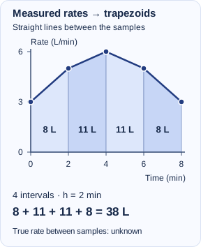
1. Join neighbouring samples with straight lines

Let $a=x_0<x_1<\cdots<x_n=b$ be sample positions, and write $f_i=f(x_i)$. There are $n$ intervals and $n+1$ sample values. The trapezoidal estimate on one interval is its width times the average of its two endpoint values:

For nonnegative values this is the area of a trapezoid. For signed values, the same expression integrates the straight-line interpolant and keeps the sign; it estimates net accumulation. Add the interval contributions. If all intervals have the same width $h=(b-a)/n$, this becomes

The endpoint weights are 1 and the interior weights are 2 when $h/2$ is factored out. Each interior sample belongs to two neighbouring trapezoids. With unequal widths, use the individual $A_i$ values; a single common $h$ would be incorrect.